Get hands-on with Elasticsearch: Dive into our sample notebooks in the Elasticsearch Labs repo, start a free cloud trial, or try Elastic on your local machine now.
Elasticsearch adds native support for OpenTelemetry exponential histograms in ES|QL. Unlike fixed-bucket histograms, exponential histograms dynamically adapt to your data — giving you accurate percentile estimates (median, p99, any percentile you want) at query time with guaranteed error bounds. No more pre-defining buckets, no more lossy conversions.
Just send your OTel metrics to the Elasticsearch OTLP/HTTP endpoint and they're stored using the new exponential_histogram type and queryable immediately. Already have historical data stored in the classic histogram type? A simple ::exponential_histogram cast in your ES|QL queries handles the migration transparently. Already using downsampling? Both histogram field types are now fully supported.
Histogram metrics
When dealing with metrics (in OpenTelemetry or Prometheus, for instance), counters and gauges are the most common metric types. Gauges allow you to monitor values that rise or fall (e.g., CPU utilization). Counters allow you to, well, count things, such as the total number of HTTP requests your service is handling. Counters normally just increase in value, with a few exceptions when they reset, like when a server reboots.
In the case of counters, you can additionally collect a counter measuring the total sum of your HTTP response times, which allows you to derive the average response time by dividing that sum by the total number of requests. However, average response times provide limited insights into the collected data and the system behavior. The best insights are gained by analyzing the collected metric distribution, e.g., through median and percentile calculations. This is where counters fall short.
In the past, workarounds have been applied: For example, classic Prometheus-style histograms attempt to capture the distribution using a set of counters. By defining fixed buckets (e.g., one for response times in the range [0s, 1s), one for [1s, 4s), and so on) and associating a counter with each, we can at least estimate percentiles broadly. However, the key problem here is that we have to know the distribution of our data up front to properly define these buckets.
To that end, the OpenTelemetry community has come up with a better solution: exponential histograms. Exponential histograms assign collected values to buckets, just like classic Prometheus-style histograms. The key differentiator is that these buckets vary dynamically based on the collected values. The name "exponential" comes from the fact that the bucket sizes increase exponentially: we use small buckets for small values and wider buckets for larger values. You can find an excellent introduction in the OpenTelemetry exponential histograms introduction.
Note that in addition to classic histograms, Prometheus also added native histograms, which directly map to OTel exponential histograms. Native histograms have their own PromQL syntax. We are actively working on adding support for that syntax to the Elasticsearch PromQL implementation, so that you can directly query exponential histograms using PromQL.
Demo setup
Let's start by collecting some histogram metrics to show how they can be stored and analyzed in Elasticsearch using ES|QL.
We'll focus on a Java JVM metric: garbage collection durations. OpenTelemetry defines the jvm.gc.duration, which is a histogram-typed metric. The OpenTelemetry Java agent natively supports collecting this metric.
We'll spin up a JVM running a Renaissance benchmark to put it under stress. We'll start that JVM with the vanilla OpenTelemetry Java agent attached and have it send the metrics directly to Elasticsearch.
You can find the ready-to-run Docker-compose file here. You'll just need to insert your Elasticsearch OTLP/HTTP endpoint and API key in the docker-compose.yml:
Note that you don't have to use this demo setup. We even encourage you to try it with your own application. Here are the other important OpenTelemetry agent settings the demo already includes, which you should include too if you're bringing your own app:
Let's step through them:
- Temporality preference: OpenTelemetry supports both cumulative and delta-based histograms. Cumulative means that the histogram is only cleared after an application restart, while delta clears it after each export. At the time of writing, Elasticsearch only supports delta temporality for histograms. We are actively working on supporting cumulative histograms as well.
- Default Histogram Aggregation: By default, OpenTelemetry exports histograms in the Prometheus-style fixed bucket format. Since we want to reap the benefits of exponential histograms, we tell the agent to use them instead.
- Runtime Telemetry enabled: This tells the agent to actually collect the detailed JVM metrics, which include
jvm.gc.duration.
Now we are ready to go! We'll let the application run in the background and switch over to Kibana to analyze the GC metric.
Querying with ES|QL
Now let's open up Kibana and navigate to "Discover". There we'll switch to ES|QL mode, and start querying the collected data:
As a response, we now see the metric panel shown below. If you don't see any data, make sure to double-check the Kibana time range filter.
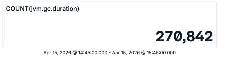
ES|QL metric panel showing the total count of jvm.gc.duration samples
This number represents the total number of garbage collection operations that happened in our test application during the selected time frame.
Similarly, we can query the total time spent on those garbage collection operations:

ES|QL metric panel showing the sum of jvm.gc.duration values in the selected time range
So we have roughly 270k garbage collections, which in total took 713 seconds. Given these two numbers, we can now compute the average if we are still fluent in primary school-level math. Even if not, you can just let ES|QL do that for you:

ES|QL metric panel showing the average jvm.gc.duration value
Now we know that the average garbage collection operation took about 3 milliseconds. However, Java experts might know that there are different kinds of garbage collections happening, which can have significantly different pause times. Fortunately the OpenTelemetry metric comes with attributes, which allow us to slice the data accordingly:
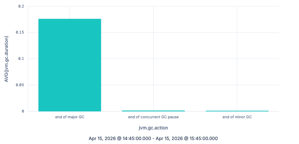
ES|QL bar chart showing the average jvm.gc.duration grouped by jvm.gc.action
As expected, major garbage collections take a lot more time per collection than minor ones, at least on average. So far, we have done nothing you couldn't also achieve by just using counters. Let's now use histograms to understand the actual distribution of the GC latency. We'll look at the data over time (by grouping using TBUCKET) and focus on the major garbage collections:
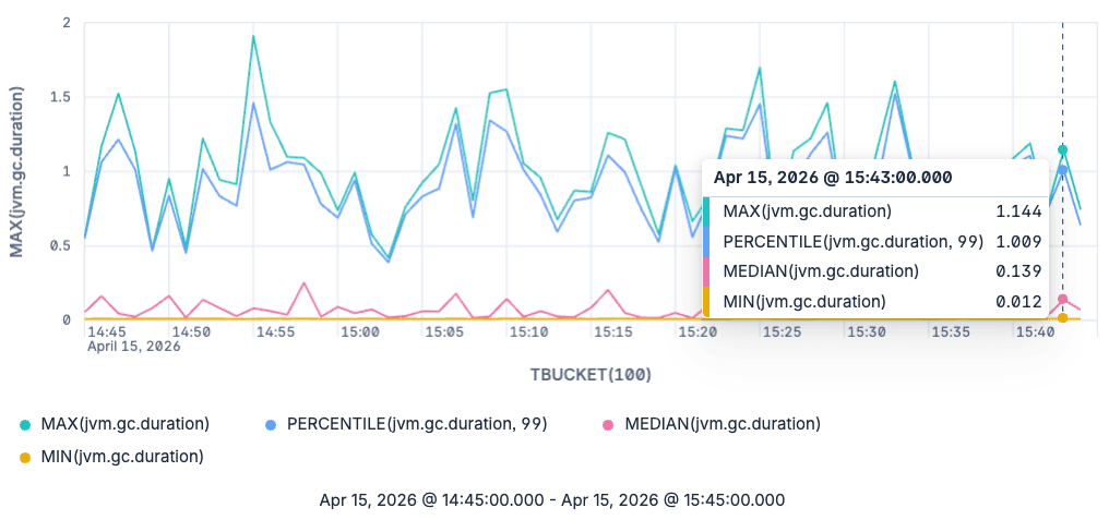
ES|QL line chart of min, median, p99 and max jvm.gc.duration for major garbage collections
The graph now shows us the minimum, maximum, median and 99th percentile for major garbage collections. Note that we aren't bound to only querying the median and the 99th percentile. We can query any percentile we'd like to see, as these are estimated at query time from the raw exponential histograms.
A note on backwards compatibility
So far, we have seen how you can use the new shiny toy in Elasticsearch and ES|QL: exponential histograms. However, since this has just reached general availability (GA) in the 9.4 release, what about your historical data?
Before exponential histograms were added, Elasticsearch was already capable of storing OpenTelemetry histograms in the histogram field type. To do so, we converted them to a different data structure supported by the histogram field type: T-Digest. T-Digest provides good accuracy for extreme percentiles (e.g., 99th percentile) at the cost of accuracy for percentiles in the middle of the distribution, such as the median. In contrast, exponential histograms provide a guaranteed upper bound on the relative error for every percentile. As conversions always introduce errors, we are happy to now have native support for exponential histograms, allowing you to collect and analyze your metrics end-to-end without unnecessary conversions.
But still, what should you do if you have historical data and still want to query it? Thanks to ES|QL union types, the answer is actually easy: You just have to add a ::exponential_histogram suffix to the histogram metrics in your queries:
When this query encounters histogram fields, it will attempt to convert them to exponential histograms. When operating on exponential_histogram fields, the ::exponential_histogram cast has no effect. Note that this also works with mixed data sets: if your backing indices use both types, the query will just do the right thing.
So if you are building queries or dashboards that you expect to run on pre-9.4 ingested data, we recommend that you simply add: ::exponential_histogram casts.
Wrapping up
Native support for OpenTelemetry exponential histograms in Elasticsearch gives you better metric fidelity and more flexible analysis in ES|QL. In this blog post, we have shown you how to easily ingest and analyze your histogram metrics with ES|QL using various aggregations and the impact exponential histograms have.
Exponential histograms are generally available in Elasticsearch basic starting with the 9.4.0 release. They will be available in Elastic Cloud Serverless a few weeks after the 9.4.0 release, once mOTLP (the managed observability OTLP intake) switches to use the Elasticsearch OTLP endpoint. We'll update this blog post and add a note on the Elastic Cloud Serverless release notes when that happens.
Frequently Asked Questions
How do I query OpenTelemetry histogram metrics in Elasticsearch?
Elasticsearch 9.4 natively stores OpenTelemetry exponential histograms and supports querying them in ES|QL. You can use standard aggregation functions like AVG, SUM, COUNT, PERCENTILE, MEDIAN, MIN, and MAX directly on histogram fields. Just send your OTel metrics to the Elasticsearch OTLP/HTTP endpoint and query them in Kibana Discover using ES|QL.
What's the difference between exponential histograms and classic Prometheus-style histograms?
Classic Prometheus-style histograms require you to predefine fixed buckets, which means you need to know your data distribution upfront. Exponential histograms dynamically adapt their bucket boundaries based on collected values, giving you accurate percentile estimates without any upfront configuration. This makes them far more flexible for real-world workloads where distributions vary.
Why are exponential histograms better than T-Digest for metric storage?
Before 9.4, Elasticsearch converted OTel histograms to T-Digest for storage. T-Digest provides good accuracy for extreme percentiles (like p99) but loses accuracy for mid-range percentiles like the median. Exponential histograms provide a guaranteed upper bound on relative error for every percentile, and native storage eliminates the lossy conversion step entirely. Also T-Digests don't support cumulative temporality.
Can I query historical histogram data after upgrading to Elasticsearch 9.4?
Yes. If you have older data stored in the classic histogram field type, you can query it alongside new exponential_histogram data by adding a ::exponential_histogram cast to your ES|QL queries. ES|QL union types handle the conversion transparently, even across mixed indices.
How do I send OpenTelemetry exponential histograms to Elasticsearch?
Configure your OpenTelemetry SDK or agent to use delta temporality (OTEL_EXPORTER_OTLP_METRICS_TEMPORALITY_PREFERENCE: delta) and exponential bucket histograms (OTEL_EXPORTER_OTLP_METRICS_DEFAULT_HISTOGRAM_AGGREGATION: BASE2_EXPONENTIAL_BUCKET_HISTOGRAM). Point the OTLP exporter at your Elasticsearch OTLP/HTTP endpoint and the histograms will be stored natively — no intermediate collector or conversion needed.
Does Elasticsearch support downsampling for histogram metrics?
Yes. Starting with Elasticsearch 9.4, both the exponential_histogram and classic histogram field types are supported in time series data stream downsampling. This lets you retain long-term histogram data at reduced storage cost while still being able to query percentiles.
How does Elasticsearch's histogram support compare to other observability platforms?
Most observability platforms either require fixed-bucket histograms (losing accuracy) or convert distributions to sketches on ingest (losing raw fidelity). Elasticsearch 9.4 stores OTel exponential histograms natively and lets you compute any percentile at query time using ES|QL, without predefining buckets or losing data to intermediate conversions.
Related Content
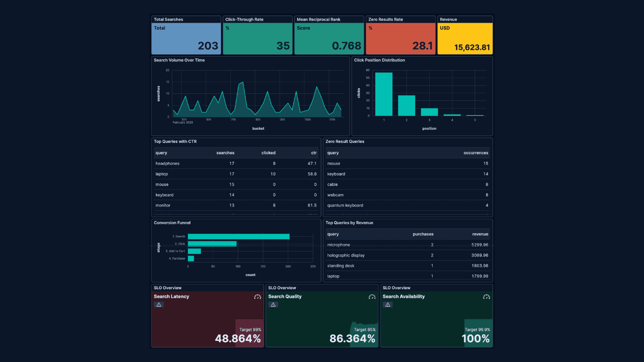
How to instrument your search API with OpenTelemetry and query it with ES|QL
Add custom attributes to OpenTelemetry spans and run six ES|QL queries that reveal your top searches, zero-result rate and slowest queries.
How to build search analytics on Elastic using OpenTelemetry, no extra pipeline required
How to instrument your search application to use modern Open Telemetry standard to drive insights in to your search and users.
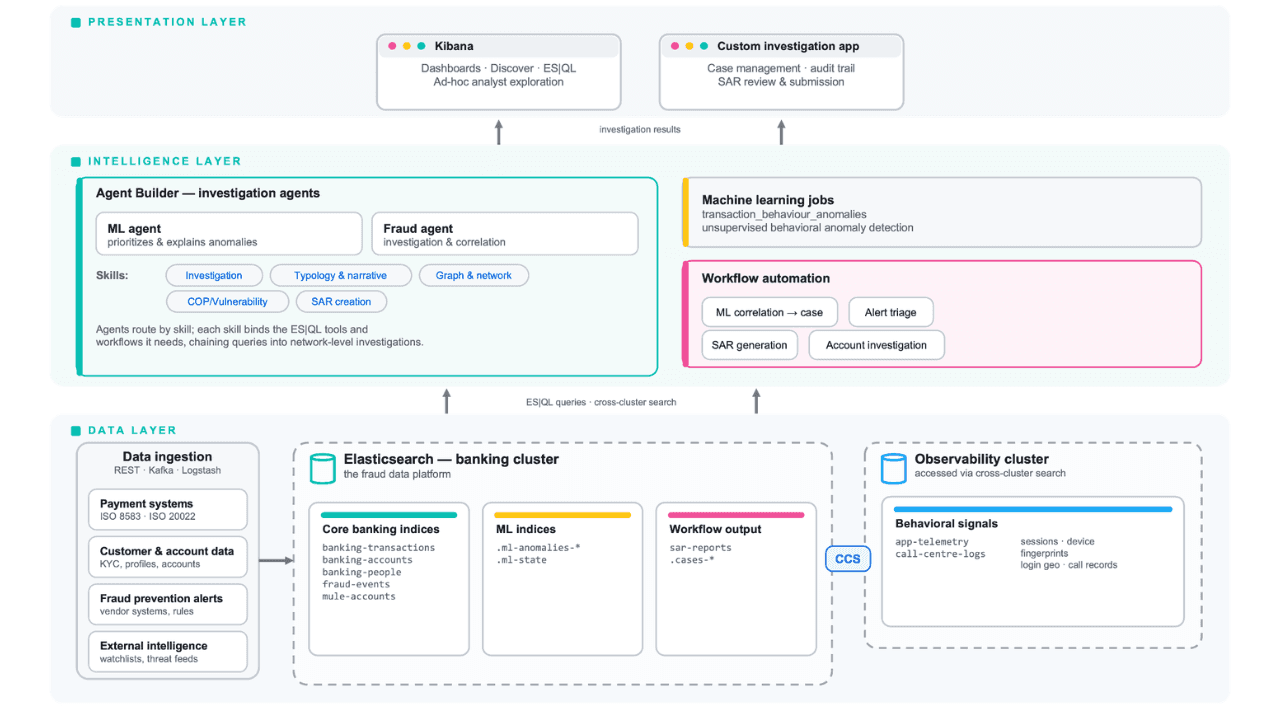
Follow the money: tracing laundering networks with ES|QL and cross-cluster search
The data model, cross-cluster architecture and five ES|QL queries that power mule detection and laundering network tracing, built from infrastructure most financial institutions already run.

July 1, 2026
One command. Natural language. Your Elasticsearch data, straight to the terminal.
Query your Elasticsearch data from the terminal in plain English. The official Elastic GitHub Copilot CLI plugin generates and runs ES|QL queries against your cluster. No Kibana, no manual syntax.
June 30, 2026
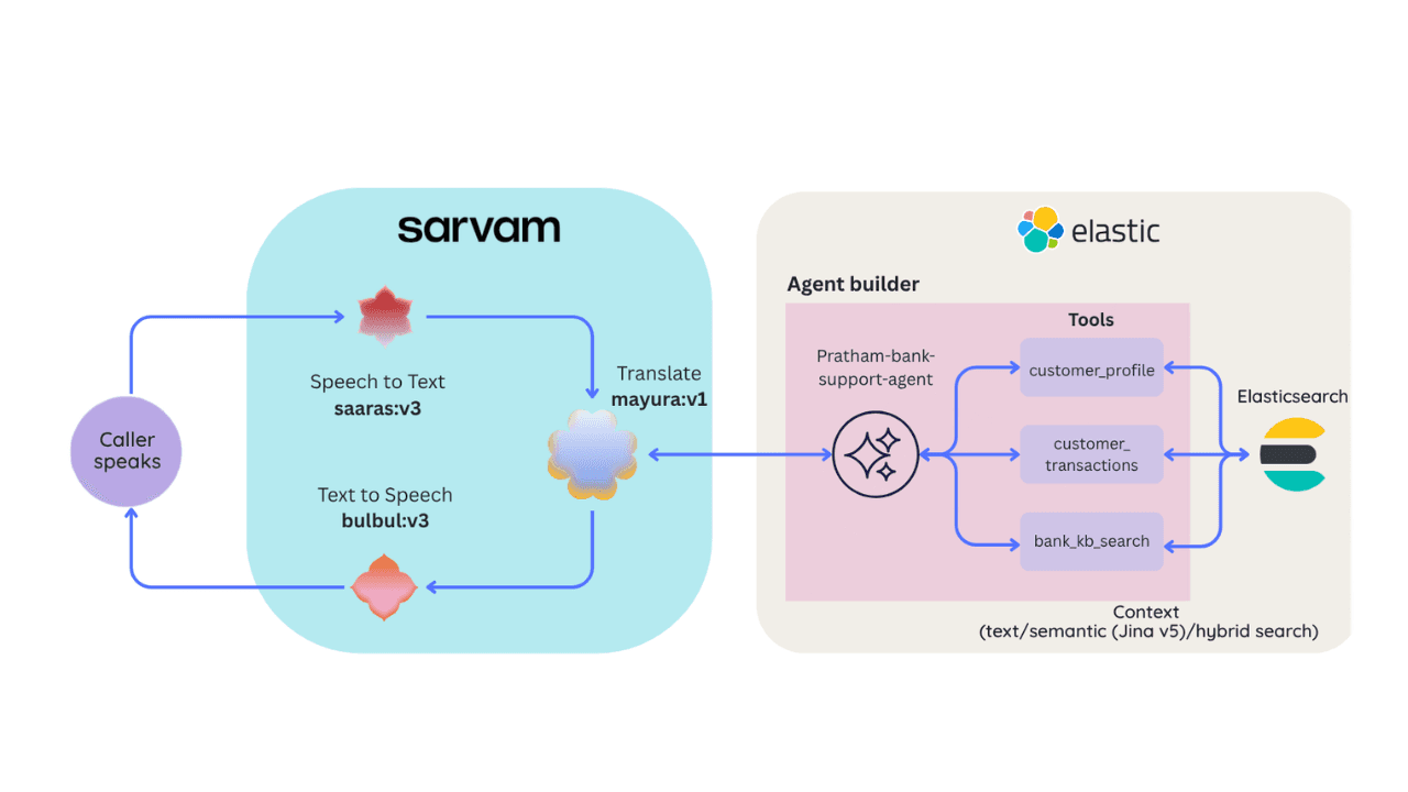
Building a multilingual voice agent with Elastic Agent Builder & Sarvam AI
A working demo combining Sarvam AI speech with Elastic Agent Builder: identity verification, per-customer ES|QL queries, and mid-call language switching across 22 Indian languages without multilingual indices.