Get hands-on with Elasticsearch: Dive into our sample notebooks in the Elasticsearch Labs repo, start a free cloud trial, or try Elastic on your local machine now.
The current generation of agentic models are remarkably good system troubleshooters. Given a hypothesis and the means to test it, they can reason about a failing service much the way a seasoned SRE does: form a theory, look for corroborating evidence, discard it when the data disagrees, and narrow in on a root cause. Their main limitation is not their ability to reason but their reach: they can only investigate what their tools let them see.
This is where Elasticsearch earns its place in the stack. It is already where a great deal of operational telemetry lives (logs, metrics, traces, events), and it exposes them through an expressive query and aggregation layer. That makes it a natural tool for an agent debugging a live system: it can slice by attribute, aggregate over time, correlate across signals, and drill from a symptom down to the documents that produced it.
We've been building an agentic layer on top of Elasticsearch that continuously monitors a system and root-causes issues as they arise. A recurring primitive in that workflow is time series event analysis. For example, given an error rate, a p99 latency, a queue depth and a throughput counter, tell me whether something happened, what it was and when. A transient spike in errors, a regime change in latency, and a step up in CPU usage are the signatures of the underlying fault, and they're typically what an agent examines first as it forms and tests hypotheses.
Elasticsearch has shipped a single-change-point aggregation for some time. It answers "did this series change?" with one verdict and the most significant change it found. That's a good fit for a dashboard, but less so for an agent, which often wants to interrogate a long window and enumerate everything of interest in it: the error spike at 02:14, the latency regime shift at 02:30, the throughput dip while the pod was being rescheduled. So we upgraded the capability to detect and report multiple events of multiple kinds in a single series. At the same time, we took the opportunity to further harden it to work reliably against whatever telemetry the agent points it at. This post describes how it works.
Why single change point detection isn't enough for agents
Concretely, we want a single entry point that takes a numeric time series and returns a small list of interesting events, each with a type, a location, a significance, and some key characteristics. We care about three classes of event, because they map onto three different kinds of underlying fault:
| Event type | What changes | Detection channel | Example fault |
|---|---|---|---|
| Structural change | Level (step) or slope (trend) shifts to a new sustained regime | Value channel | Config push doubles baseline latency; memory leak turns a flat curve into a ramp |
| Distribution change | Noise level (variance) shifts while the mean holds steady | Dispersion channel | Service responds erratically at the same average latency |
| Point anomaly | Isolated spike or dip against a stable background | Value channel (pulse detector) | Single burst of errors; one-minute throughput drop during GC pause |
The hard part is not detecting any one of these on clean, well-behaved data. The hard part is doing it on arbitrary telemetry without per-series tuning. The agent does not know in advance whether the series it is examining is near-constant, smoothly drifting, heteroscedastic (quiet in places and noisy in others), sparsely populated, or has a magnitude of . It is not scalable to hand-pick parameters for every series it needs to analyze. Whatever we build has to be robust to all of that while maintaining excellent recall and precision. If it fails to detect important events it runs the risk of missing key corroborating evidence for a working hypothesis. Conversely, an analysis tool that reports an event for every minor fluctuation will pollute the context the agent reasons over.
The design goals, in priority order, are: correct on diverse data out of the box, parsimonious (report only what matters), and cheap enough to run interactively across many series.
How PELT and BIC power change point detection
Change-point detection is a well studied field. The classical offline formulation searches for the segmentation of a series that minimizes a penalized cost: a per-segment goodness-of-fit term plus a penalty for each added break to stop the optimizer from putting a boundary between every pair of points. Solved naively, this is combinatorial, but PELT (Pruned Exact Linear Time, Killick et al.) finds the optimal partition in roughly linear time by using a dynamic program to prune candidate boundaries that can never be optimal. On the labeling side, comparing nested models by an information criterion such as the Bayesian Information Criterion (BIC) gives a principled, scale-aware way to decide whether a candidate break is really important and what sort of change it constitutes.
These are good building blocks, and we use them. However, the textbook recipe assumes more than telemetry gives you. It typically assumes a single change type (a mean shift), a known and stationary noise level, and reasonably benign numerics. Real telemetry violates all three: variance changes matter as much as mean changes, the noise level is unknown, often heavy-tailed and changing, and the data spans extreme magnitudes and degenerate cases, such as perfectly constant segments, that wreck an ill-conditioned polynomial fit or a fixed-variance cost. Most of the engineering I describe below is about closing that gap.
Splitting one time series into three detection channels
Rather than trying to find one detector that does everything, we run three focused detectors and then merge their findings. Two of the three are the same structural detector applied to two different views of the data, or channels.
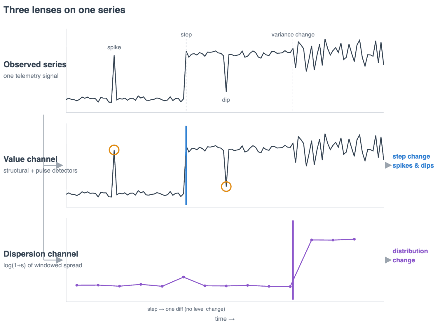
One observed series is read by a value channel (for structural step/trend detection plus point spike/dip detection) and a dispersion channel (for distribution-change detection on a windowed measure of spread). A step appears as a level shift the value channel flags and as a single large first difference the dispersion channel ignores; a variance change is invisible to the value channel but creates a step in the dispersion channel.
Two detectors run on the value channel: a structural detector that flags step and trend changes, and a pulse detector that identifies point spikes and dips. The dispersion channel, a windowed measure of spread, is fed to a second copy of the structural detector, where a variance change shows up as a level shift and is relabeled a distribution change. The two channels are complementary by construction: a step is a level shift the value channel flags but only has a single large first difference the dispersion channel ignores, while a variance change is invisible to the value channel yet shows up clearly in the dispersion channel. A thin orchestration layer then merges and de-duplicates the streams.
Keeping the three concerns separate makes each one tractable. A mean-shift detector and a variance-shift detector pull in opposite directions if you try to fuse them; a point-anomaly detector and a regime detector need opposite robustness settings. Separated, each can be tuned to its job.
PELT with a scale-free cost
For the structural channel, we fit each candidate segment with a low-order polynomial (constant or linear) and score it with the profiled-variance Gaussian cost. If a segment of length has residual sum of squares , the cost is
This is the negative log-likelihood of a Gaussian segment after profiling out the variance, i.e., after substituting the maximum-likelihood estimate back into the log-likelihood. The total objective PELT minimizes is the sum of segment costs plus a per-break penalty,
Here, is the BIC complexity term (number of parameters times where is the number of values in the time series) and the scale factor lets us trade sensitivity against parsimony in one place.
Using the profiled cost rather than a cost against a fixed global variance is a deliberate and important choice. The global noise level of telemetry is unreliable: on a smoothly varying series the natural estimate (the spread of first differences) can collapse toward zero, and a fixed-variance cost then treats every wiggle as enormously significant and over-segments. The profiled cost depends only on the ratio , so it is invariant to the absolute scale and immune to that failure. A small floor on keeps the logarithm finite, so a zero-residual segment is not rewarded without bound.
Keeping the fit stable using robust local weighting
Before PELT runs, we robustly down-weight points so that an excursion does not create spurious breaks or drag a segment boundary onto itself. Crucially, these weights enter into the weighted residual moments, so they shape not just the segment fit but its residual variance, and so the segment costs themselves. Each point gets a Cauchy weight, , of its residual from a rolling-median baseline against a robust scale : points near the local median keep full weight and points far from it are progressively discounted. A nice side effect of measuring excursions from the median on a window centered on each point is that clean structural breaks do not get down-weighted at all, because the majority of values land on the same side of the break as the point whose residual is being computed. So a sustained regime keeps full weight, but a lone spike does not.
There is a nice justification for scoring a weighted Gaussian cost when what we really want is robustness to a heavy tail. The Cauchy weight is exactly the iteratively reweighted least squares (IRLS) weight of its loss: , so the weighted normal equations are identical to the Cauchy M-estimator's estimating equations . A weighted-mean (or weighted-line) fit at those weights is therefore a Cauchy M-estimate, not a Gaussian one. The cost we actually evaluate inherits the same properties. Because is concave in , its tangent at the current residual lies above it. This gives a pointwise bound with the weight at the tangent point; summing, the weighted residual sum of squares is a tangent upper bound on the total Cauchy loss, touching it in both value and gradient at the weights' anchor point. Minimizing the weighted RSS is thus one step of a majorize–minimize scheme that provably decreases the true Cauchy objective, and the profiled-variance cost we feed the BIC is that majorizer standing in for the Cauchy deviance. The only approximation is that we anchor the weights once, at the rolling-median baseline, rather than iterating IRLS to its fixed point; this is exact for the inliers that sit near the baseline, and correct for gross outliers, whose vanishing weight removes them from the cost wherever the bound is loosest.
Finally, the trick that makes this work on heteroscedastic data is that the residual is judged primarily against a local robust scale, not a global one: the MAD of residuals in the same sliding window. On a series that is quiet in one stretch and noisy in another, this means a spike in the quiet stretch that is multiple local sigmas is correctly suppressed. The local MAD can collapse on quiet stretches, so we use a backstop that is a fraction of a global composite of robust scales and a floor related to the quantization error for discrete series and numerical precision otherwise.
From candidates to labeled events using BIC verification
PELT gives a globally optimal penalized segmentation, so we take its boundaries as candidates and verify each one. For a candidate at index we look at the window of length spanning to its nearest neighboring candidates and compare a no-change null against step and trend alternatives by BIC,
where counts the fitted parameters (the same parameter count as in the PELT penalty above). We map the BIC gain of an alternative over the null to a significance via , to turn a threshold into a decision boundary). We treat this as a significance score for ranking and thresholding, not as a calibrated tail probability.
At this stage we allow higher-degree models to avoid splitting smoothly varying trends. These are problematic in PELT itself because it considers short segments, which they overfit. We keep the most parsimonious alternative that clears the significance threshold and survives a persistence check. The persistence check re-scores with the weights immediately around the candidate muted, and if the evidence collapses, the "change" was driven by a few extreme points – an excursion, not a regime change – and we reject it. The polynomial order is applied symmetrically to the null and to each side of the split, so the alternative is always the same model class merely split at the candidate, and therefore strictly more flexible. The whole process can be thought of as Bayesian model selection with a preference for the null.
When no candidate survives, we still say something useful: we report the series as "stationary" (best no-change model is a constant) or "non-stationary" (best model has a slope), with the trend direction. For an agent, "this series is cleanly trending up over the window" is itself a finding.
Detecting distribution changes with a dispersion channel
A variance change is indirectly visible to the mean channel – worse, the robust weighting there actively mutes the excursions that signal it. So we detect it on a separate dispersion channel and reuse the exact same structural detector, because on this channel a variance change is just an ordinary level change.
The channel is built from one sample per non-overlapping window. Within a window, we take the inter-quartile range of the first differences, rescaled to a standard-deviation equivalent (), and pass it through :
Then . Three choices matter here. First-differencing cancels level and slope, so a mean step contributes a single large difference rather than inflating the whole window, and a steady ramp produces a flat channel. Non-overlapping windows keep the samples independent; overlapping windows autocorrelates the channel and makes the segmenter over-detect. And the IQR is used rather than the median (which is too robust and will miss a window that is 40% noisy then flatlines) or the raw standard deviation (which is not robust enough since one spike's two large differences inflate the window). Because the dispersion channel is a fraction of the original length, the verifier there is restricted to a lower-order null so a genuine low-high-low variance bump is not absorbed.
The functional form is worth dwelling on, because each part earns its place. The log makes the channel respond to ratios of noise level rather than absolute differences. Variance changes in telemetry are typically multiplicative: a regime is "twice as noisy". On a raw-scale channel, a doubling shows up as an enormous absolute jump at a high baseline and a negligible one at a low baseline, so an additive step-cost detector would find variance changes trivially in loud series and miss them in quiet ones. Under a log, a factor- change in scale is the same offset wherever it occurs, which is exactly the additive-step behavior the structural detector is built for. The " is a soft floor. A bare diverges to as the scale goes to zero, which is precisely what happens on a near constant stretch, and would manufacture a huge spurious step at the first noisy window after it. Conversely, is finite and smooth at zero, behaves linearly () while the noise is small, and recovers the multiplicative behavior once the noise is appreciable. This gives graceful degradation instead of a singularity, and with no tuned epsilon to pick. Note that squaring the scale (using a variance instead) only doubles the dynamic range; it makes no difference to the detector either way, since differs only by a constant the threshold absorbs.
Detecting point anomalies as excursions from a local baseline
Spikes and dips are detected as point excursions from the local rolling-median baseline. Working from the local residual rather than raw values means level structure is removed and smooth curvature is tracked; even for time series that change significantly the detector is sensitive to significant local deviations.
The pipeline is a generous proposer followed by a strict gate:
- Propose every point whose residual exceeds a threshold number of robust sigmas. The scale is the larger of the global first-difference noise (which stays meaningful on smooth data where most residuals are exactly zero) and a composite of robust scales of the residuals (which inflates once a frequent large-residual population appears).
- Merge adjacent same-sign candidates into excursions, dropping any that span a full minimum segment: that is a regime, and is owned by the structural channels.
- Rank and cap the excursions by peak z-score, keeping the top , so a pathological series cannot drown the output.
- Gate using one shared null: build a Gaussian KDE from the series with all of the retained excursions removed, and keep an excursion only if its peak's Bonferroni-corrected upper-/lower-tail probability under that null clears the threshold.
Removing all the tested excursions from the single null at once is a key trick. The leave-one-out alternative – score each excursion against a null containing the others – lets the largest spike and dip mask everything else. Removing them together means several genuinely distinct excursions are each judged against the remainder and all survive, while a recurring population is still rejected.
The proposer and the gate ask deliberately different questions, and that distinction drives two further choices. The proposer works on residuals from the rolling median since it wants recall, and a residual is what tells you a point stands out from its local neighborhood. The gate is value-based: it asks "is this magnitude one we see at other times in the series?", so a spike to a level that recurs elsewhere — such as periodic batch jobs — is suppressed even though it is a large local residual. Those are the right semantics for an agent, but they expose a heteroscedasticity problem, because telemetry noise is almost always a function of magnitude. Periodic spikes can sit orders of magnitude above the background, and a single KDE bandwidth fitted to the whole value range is then far too narrow up in the high tail. So ordinary large values come back as significant, a steady source of false positives.
The fix is a variance-stabilizing transform. We run the value gate in space, where is a robust measure of the spread of the background. is linear for and logarithmic for , which turns a multiplicative (magnitude-dependent) spread into a roughly constant one, so a single bandwidth is valid across orders of magnitude. It is also odd and finite at zero, so exact zeros and sign changes (dips below a small baseline) need no special handling, unlike a bare log. Crucially, it is monotone and so does not change what is tested (for any monotone function , ) so it only fixes the estimate of that tail probability.
One subtlety closes the loop. The KDE null and the kernel bandwidth are taken from different scales, on purpose. The null is the stabilized background values: so it models any mode in the data, which is what makes a recurring large magnitude unsurprising. However, the bandwidth is taken from the stabilized residuals, not the stabilized values, because a genuine level change makes the value distribution bimodal, and a bandwidth computed from that bimodal spread would balloon, masking a real spike sitting on top of a shifted regime. The residual removes the step, so the bandwidth always reflects within-regime noise and the gate stays sensitive to a deviation that is extreme relative to its own neighborhood if it is also outside the envelope for the series as a whole.
Merging structural, distribution, and point anomaly events
Finally, an orchestration layer merges the structural, distribution, and point-anomaly event streams. Structural and distribution events that mark the same regime boundary are de-duplicated to the more significant one (a boundary that shifts both level and spread is one event, not two). Pulses are a separate stream added after de-duplication, because a spike that lands on a structural boundary is a real, separate finding and must not be suppressed. Everything is then mapped back from the internal value-array index space to source-bucket indices.
Handling extreme magnitudes and edge cases
What makes this usable as an unattended tool is a collection of defensive choices for the cases that break naive implementations:
- Variance computed as loses all precision at large magnitudes: a constant series at can manufacture phantom change points purely from floating-point error. We center every PELT input by a constant offset first; the polynomial RSS is invariant to that shift in exact arithmetic, but the working magnitudes drop from to .
- Using raw indices as the regressor results in poor condition polynomial fits: the largest moment is , which is about for a cubic over a 2000-point window. This trips the SVD singularity guard and silently degrades the fit. Mapping affinely onto leaves the fit identical (RSS is invariant under reparametrization) but every moment becomes .
- Scale-free cost, as described, means the segmentation cost doesn't depend on tuning a noise estimate.
- Down-weighting wants a primarily local scale: suppress whatever is anomalous in its own neighbourhood. It uses the maximum of MAD and a small global floor on the differences from the rolling median. Conversely, spike/dip detection wants a global scale: we care about global outliers. It uses a composite of robust scales of all differences. Using the wrong one in either place produces characteristic failures – irrelevant spikes in a quiet segment, or locally large excursions creating spurious breaks – and maintaining separate channels allows us to pick appropriately.
- Using one p-value threshold, Bonferroni-corrected by the number of candidates, applied consistently across all three detectors, means that "how surprised should I be" is consistent everywhere.
The recurring theme is that the difference between a detector that works in a notebook and one that works on a firehose of production time series is mainly in handling the edge cases gracefully.
Performance: ~1ms per series on a single core
Detection cost is dominated by PELT. Its segment cost is a profiled-variance linear fit, which we evaluate in constant time from prefix-summed weighted moments rather than maintaining a regression per candidate boundary, so a single segment cost is a handful of array reads and a 2×2 solve. Cost grows a little faster than linearly with series length since PELT's pruned candidate set does not stay constant on noisy data. Therefore, to bound the worst case on very long series, we downsample ahead of detection: above a cap (2000 samples), the series is collapsed into macro-buckets, keeping two samples per bucket: the median and the largest local deviation. This is inspired by the M4 downsampling scheme, but because we need only the median and the largest excursion for structural-change and outlier detection, respectively, we can then afford to double the bucket resolution. The downsampled series carries its original bucket indices, so every reported event still maps back to a real source bucket; below the cap it is a no-op. The whole analysis is a single pass over the (possibly downsampled) series with no per-series configuration. This lets the agent call it freely across many signals.
In absolute terms, this means the analysis is comfortably interactive. On a single core, post-warmup, a typical series of 140–350 buckets is analysed in about 1 ms (≈220,000 buckets/s), and a series long enough to hit the downsample cap (say 5,000 buckets, collapsed to 2,000) takes about 40 ms, which is the effective worst case per call. For an agent issuing a handful of these calls per investigation, and parallelising across the many series in a `BY` query, the latency is negligible.
Evaluation on synthetic and production telemetry
Synthetic benchmark
We evaluate first on a synthetic generator with known ground truth, because it lets us measure the things that matter precisely. The generator produces random time series with diverse behaviors, which we group into three families. The positive family injects known events of each type: clean and noisy step changes (up and down, SNR around 10, at several positions), trend onsets and ramps (including a flat–ramp–flat sequence with two boundaries), variance changes with a constant mean (single steps and a low–high–low bump), and isolated spikes and dips. The null family ideally produces no event: stationary noise, perfectly constant series, smooth quadratic drift and clean ramps, and periodic signals. (A variance change with a constant mean is not null: it is a distribution change, an abrupt step on the dispersion channel, and so it belongs in the positive family above. The related null requirement, that such a change does not surface on the value channel as a step, is checked separately.) The adversarial family stresses the robustness machinery: a perfectly flat series at a magnitude of (for which a naive variance arithmetic manufactures phantom breaks here through catastrophic cancellation) and, conversely, a genuine spike or step in a noisy baseline as high as (which must still be found and located, the high baseline notwithstanding); a spike on top of a step; a within-regime spike after a 100 level jump; a recurring train of equal peaks (a population, not individual spikes); wide sustained excursions (a structural change, not a spike or dip); and fuzzed random level-shift series. On these series we track recall per event type, precision and the false-positive rate on the null family, localization error, parsimony (events per series and adherence to the count limit), and invariance under constant offsets, rescaling and extreme magnitudes.
The table below summarizes what the suite tests.
| Event family | Representative scenarios | Required outcome | Localization tolerance |
|---|---|---|---|
| Step | clean / noisy, up / down, single and multiple, several positions | detected | ≤ 4–8 buckets |
| Trend | slope change and flat–ramp–flat, clean and in noise | detected | ≤ 8–12 buckets |
| Distribution | variance step (mean constant), low–high–low bump | detected | ≤ 1 dispersion window |
| Spike / dip | isolated, multiple distinct, on heavy-tailed and high-magnitude series, within-regime after a step | detected, capped at max(5, 2% of n) | ≤ 2 buckets |
| Null series | stationary noise, constant, smooth drift / ramp, periodic | no event reported | n/a |
| Invariance / robustness | constant offset, rescaling, 10^5–10^9 magnitudes, spike-on-step, recurring population, wide excursion | result unchanged / no spurious event | n/a |
Running this over 400 series per scenario, just over half a million buckets in total, and scoring with the same two categories we use for the real-data evaluation below (any regime change versus point spikes and dips) gives:
| Event type | Recall | Precision | Median localization error |
|---|---|---|---|
| Structural change | 0.994 | 0.664 | 0 |
| Spike / dip | 0.847 | 0.746 | 0 |
Two things stand out. When an event is detected, it is placed essentially exactly: the median localization error is zero buckets for both categories; and the point-wise accuracy, 0.998, is directly comparable to the 0.995 we report on real telemetry below: the overwhelming majority of buckets are correctly left unmarked.
The precision figures are lower than on real data, and understandably so. A sixth of this population is a hostile null family (periodic signals, smooth drift, clean ramps) chosen precisely because they tempt a detector into a spurious break, and every false alarm on them counts against precision. The resulting false-positive rate is 0.5% per bucket, with 15% of null series carrying at least one spurious event. We treat this as the conservative end of the range: on the real-telemetry mix below, where the null series are less adversarial, precision rises to 0.85 (structural) and 0.90 (spikes/dips). Finally, offset and scale invariance holds on all 400 series: the same events, to within a few buckets, whether the series is shifted by a constant or rescaled by up to three orders of magnitude.
That raw precision also misses how the result is consumed. The agent reads events most-significant-first, so a false positive only does harm if it outranks a genuine one, and by and large it does not. The median p-value of a true positive is about , against about for a false positive: the genuine events are typically overwhelmingly more significant. Concretely, if we keep only the top events per series by significance (with the true count) precision rises to 0.94, and a randomly chosen true positive is more significant than a randomly chosen false positive 93% of the time. It is not a perfectly clean separation: a strong periodicity or a sharp curve genuinely can contain a significant-looking break, which is why that figure is 0.94 rather than 1. However, the ranking is reliable enough that an agent reading from the top, or applying a stricter significance cut-off, sees the real events first and the false alarms as a lower-significance tail. This is also why exposing the detector's significance to the agent (see What's next) matters more than squeezing the raw precision higher.
Real cloud telemetry
To evaluate on real data, we scraped around 300 metrics from our production cloud environment. These cover HTTP status-code counts, failed memory allocations, memory usage, network usage, page faults, CPU usage, and throttling metrics, measured both per instance and aggregated across the fleet as a whole. Their values range over more than 12 orders of magnitude, and they display a variety of behaviors including ramps, periodicity, step changes, distribution changes, and trend changes. The figure below shows a sample of series together with the detections we make on them.
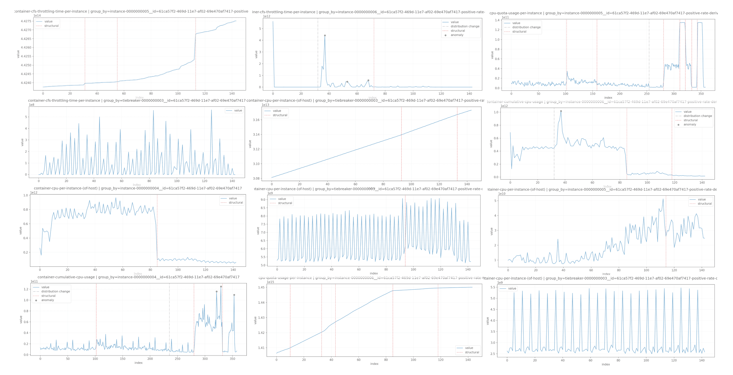
Example telemetry time series together with their change, spike and dip detection results
To get a sense of the accuracy on this set data, we labeled a subset of 150 most interesting time series, marking the visually clearest features in each. This labeling is not necessarily optimized for our target use case, where false negatives are typically more problematic than false positives: an agent consumes these results as part of a broader investigation and can pull additional information to corroborate them. Even so, we find excellent agreement with human judgment on these series. Since each series comprises between 140 and 350 points, the point-wise accuracy, at 0.995, is extremely high: the great majority of points are correctly identified as neither a change, a spike, nor a dip. But the more telling metrics are recall and precision on the human-labeled points, shown in the table below. The human labels did not attempt to categorize each change, so we break the results down only into "structural changes" and "spikes / dips" — the same two categories, and the same point-wise accuracy and recall/precision metrics, as the synthetic benchmark above.
| Event type | Recall | Precision |
|---|---|---|
| Structural change | 0.94 | 0.89 |
| Spike / dip | 0.97 | 0.92 |
It is worth covering exactly why we get disagreements. These largely fall into three categories: spikes and dips in context, isolated breaks, and small-magnitude breaks in stable series. We deliberately do not try to detect spikes and dips that are unusual only in their immediate context; that is, not globally unusual but visually significant relative to an inferred periodicity in the data, for example. Trying to account for these without fully modeling the seasonality in the data hurt precision more than it helped recall, and we have a separate persistent anomaly-detection process that builds more complete models of baseline behavior over time. Isolated breaks are an artifact we decided to live with: PELT's cost function tends to isolate a change point with a few values intermediate between the two regimes, because absorbing it into either neighboring span inflates that span's cost. Humans are good at judging such situations visually and assign a single change point. Finally, small-magnitude changes are simply not visually obvious. We detect them deliberately and regard this as a strength of a quantitative approach, since they are often the early precursors of an incident whose later, larger effects drown them out.
How the agent uses change point results in ES|QL
To the agent, all of this is one tool call: it points it at a collection of time series and gets back a typed, located, ranked list of events. That list is small by construction, which means it drops cleanly into the model's context without crowding out everything else it is reasoning about. Because the result contains multiple events, a single call over a window can hand the agent the whole local story – "error spike at 02:14, latency regime change at 02:30, throughput dip at 02:31" – and let it correlate across signals to a root cause.
Operationally, we expose this through both the ES|QL CHANGE_POINT command and the change_point aggregation. Currently, we have not extended the change_point aggregation to return multiple change points since it breaks backwards compatibility of the output schema. It just returns the most significant event. We don't have the same restriction for ES|QL since it returns change points annotated onto the table rows to which they apply. We do plan to revisit the output schema for both ES|QL and the aggregation in a later version. We'd like to migrate to optionally returning significance in log-space, which doesn't underflow, and including a short verbal description of each change, which we expect to help agents when seeing just the change points themselves.
ES|QL is Elasticsearch's piped query language, and CHANGE_POINT runs the detector as one stage in a pipeline. Its BY clause enables it to analyze many series at once (one per group) so the agent can, in a single query, segment every service's latency or every host's error rate side by side rather than issuing a call per series. The actual leverage, compared to the change_point aggregation, is composability: the events come back as ordinary rows in the pipeline, so the agent then has the entire ES|QL language to manipulate them downstream. It can filter to a window, join change points against deploy markers, count events per service, rank by significance, feed the survivors into a further aggregation, and so on.
For example, suppose the agent wants to find out whether any servers have recently seen a sudden CPU spike or a prolonged step change in CPU usage over the last 12 hours, and whether that might point to a load-balancing issue. It could use the following query:
Here it's using a STATS ... BY host.pod to see how the detected events cluster across other dimensions of the data, such as the Kubernetes pod, and so judge whether they share a common cause.
What's next for ES|QL time series analysis
As far as detecting events of interest in time series, the foundation is in place: a single, robust, parsimonious tool that turns a raw telemetry series into the short list of events that actually matter, which is exactly the kind of reach an agentic SRE needs. Going forward, we plan to explore the best mechanism for feeding the detector's uncertainty to the agent, so that a borderline event can be flagged as "worth a second look" rather than silently included or dropped. Also, this is the first of several analytical tools we plan to build into the ES|QL query language to enable agents to triage and RCA issues more effectively; so stay tuned for further updates.
Related Content

How to instrument your search API with OpenTelemetry and query it with ES|QL
Add custom attributes to OpenTelemetry spans and run six ES|QL queries that reveal your top searches, zero-result rate and slowest queries.