Try out vector search for yourself using this self-paced hands-on learning for Search AI. You can start a free cloud trial or try Elastic on your local machine now.
In CPU vector search, Elasticsearch's Optimized Scalar Quantization (OSQ) (the algorithm behind Better Binary Quantization (BBQ)) beats TurboQuant where production systems care most: throughput, ranking accuracy, and storage efficiency. In our tests on Apple M2 Max, OSQ's symmetric kernels are 10-40x faster, and on shifted embeddings its 1-bit document encoding beats TurboQuant at 4 bits on ranking accuracy while using far less storage. TurboQuant still wins on raw reconstruction MSE, but that advantage comes mostly from the Hadamard rotation and does not translate into better CPU search behavior.
A brief quantization primer
Vector search indexes often store millions or billions of embedding vectors, each hundreds or thousands of floats wide. Scalar quantization compresses each float coordinate independently to a small integer, typically 1, 2, or 4 bits, reducing storage by 8-32× and enabling fast integer-arithmetic scoring.
Why does per-coordinate quantization work at all? Because the expected squared error decomposes as a sum of independent per-coordinate terms: , by linearity of expectation. Each coordinate can be quantized independently regardless of the joint distribution. The remaining question is how to make each per-coordinate quantizer good.
BBQ and Optimized Scalar Quantization
Better Binary Quantization (BBQ), and its underlying algorithm Optimized Scalar Quantization (OSQ), have been part of Elasticsearch for multiple releases. OSQ is an evolution of several techniques to make scalar quantization more accurate, specifically for vector search.
Each vector's components are mapped to a uniform grid over an interval . The interval is initialized from the vector's statistics (assuming approximately normal residuals), using the exact same optimization objective as TurboQuant but with an additional constraint on centroid positions. They are then refined by coordinate descent to minimize an anisotropic loss , where is the quantization error vector. With the production default , this deliberately sacrifices some MSE to concentrate accuracy along the query direction. This is the direction that matters for ranking.
Before quantization, the segment (or cluster in the case of Inverted Vector File (IVF) indices) centroid is subtracted from every vector. This removes the dominant shared component that would otherwise waste the quantizer's dynamic range. Both the symmetric and asymmetric dot-product paths also center the query using the same segment centroid, so the only quantized inner product is between centered residuals. The correction terms, for each vector and , depend on only a single vector each, and can be precomputed exactly. Centering therefore adds no per-pair cost.
Documents are quantized at 1-bit (32× compression), queries at 4-bit (cheap since there are only a handful per search). The storage constraint binds on documents, not queries, so spending more bits on the query side recovers float-query accuracy while keeping per-document footprint minimal.
A block-diagonal orthogonal preconditioner equalizes coordinate variances and normalizes their distribution before quantization. This is the same goal as a full Hadamard rotation used by TurboQuant, but with no power-of-2 padding overhead.
Because the grid is uniform, quantized dot products decompose into integer dot products with scalar corrections. This enables NEON/SVE and SSE/AVX popcount and multiply-accumulate pipelines: bit-plane decomposition for 1-bit and 2-bit, nibble multiply for 4-bit, and a RaBitQ-style mixed 4×1 kernel that decomposes to four 1-bit kernels.
For a deeper dive into the sparse rotation and what it brings to robustness, see the Robust Optimized Scalar Quantization blog. For a full walkthrough of optimized scalar quantization, see this OSQ deep dive.
TurboQuant
TurboQuant (Google, ICLR 2026) takes a slightly different path to the same starting observation: that concentrated, predictable per-coordinate distributions are easy to quantize well.
Rather than adapting the quantizer per vector, TurboQuant normalizes the vector and applies a shared randomized Hadamard rotation to the entire dataset. This general sort of idea was first proposed and formalized by RaBitQ, which showed that the random rotation yields worst-case bounds over the data, holding for any fixed unit vector, for their quantization scheme. The idea of implementing via a Hadamard rotation was suggested by Weaviate for rotational quantization. After normalization and rotation, each coordinate's distribution almost always converges to in high dimensions, regardless of the original data. TurboQuant builds on this foundation: with the distribution pinned down, it solves for the optimal Lloyd-Max scalar quantizer, a 1-D -means problem on the known density. The resulting non-uniform centroids bunch up where the density is highest (near zero) and spread out in the tails. This achievies provably near-optimal MSE: within ~2.7× of the information-theoretic lower bound in general, and as tight as 1.45× at 1-bit.
For inner products, MSE-optimal quantizers introduce a multiplicative bias (which is most severe at 1-bit: ). TurboQuant corrects this with a two-stage design (): spend bits on the MSE quantizer, then use the remaining 1 bit for a Quantized Johnson-Lindenstrauss (QJL) sketch of the residual, yielding a provably unbiased inner-product estimator.
The paper's nearest-neighbour experiments were conducted on GPU (NVIDIA A100), where the lookup-table access pattern maps naturally onto shared memory.
The key design divergence: integer arithmetic vs. lookup tables
The difference between uniform and non-uniform centroids may seem minor, but it creates a large computational gap.
OSQ's uniform grid means each quantized coordinate is an integer whose arithmetic meaning is preserved. The dot product of two quantized vectors decomposes into an integer dot product, directly exploitable by SIMD: vpdpbusd on x86, multiply-accumulate and vcnt (popcount) on ARM NEON. The pipeline is branch-free and the data access pattern is sequential.
TurboQuant's non-uniform centroids break this. Each coordinate pair requires looking up a centroid value from a shared codebook, and the access pattern is data-dependent with each index selecting a different table entry. On NEON, which lacks a float gather instruction, this means scalar loads to build each vector register before the Fused Multiply-Add (FMA). Precomputing per-coordinate product tables ( entries, amortized over all documents) doesn't help either: the FMA is relatively cheap on modern cores, so the bottleneck remains the data-dependent gather, not the arithmetic. Our benchmarks confirm this: precomputed ADC tables are no faster (and sometimes slower due to the larger working set) than inline centroid lookup.
Terminology
The results sections below refer to several OSQ scoring configurations. All use uniform-grid quantization with scalar correction terms to recover the exact dot product up to quantization noise.
Symmetric -bit quantizes both query and document at bits per coordinate.
Asymmetric keeps the query as a full float vector and quantizes only the document. The dot product is a float-times-integer sum. This is more expensive per pair than symmetric, but avoids any query quantization noise. TurboQuant's scoring is always asymmetric (float query dotted against quantized document via centroid lookup).
1-4 is the production configuration for OSQ: documents at 1-bit (32× compression), queries at 4-bit. This exploits the asymmetry of search: there is one query but millions of documents, so query storage is free but document storage is the binding constraint.
Centered means the segment centroid has been subtracted from all vectors (and the query) before quantization, with the exact correction recovered from precomputed scalar terms. Centering focuses the quantizer's dynamic range on the information-bearing residual rather than the shared mean.
controls the anisotropic loss tradeoff: minimizes pure MSE, (production default) sacrifices some MSE to concentrate accuracy along the query direction, the direction that determines ranking.
How do they compare in practice?
The following results were obtained on an Apple M2 Max. The code to reproduce all these results is available here.
Head-to-head: MSE
On reconstruction MSE, the metric TurboQuant was designed to optimize, TurboQuant outperforms plain OSQ at every bit-width.
Relative MSE () on Gaussian vectors (1,000 vectors, lower is better):
| Bits | OSQ (λ=0.1) | OSQ (λ=1) | TurboQuant | TQ vs OSQ ($\lambda=1$) |
|---|---|---|---|---|
| 1 | 0.512 | 0.362 | 0.307 | 1.18× |
| 2 | 0.138 | 0.118 | 0.092 | 1.28× |
| 3 | 0.038 | 0.037 | 0.026 | 1.42× |
| 4 | 0.011 | 0.011 | 0.007 | 1.61× |
The columns reveal that OSQ's production setting () deliberately sacrifices MSE for dot-product accuracy. With (pure MSE), the gap narrows, to just 1.18× at 1-bit.
But where does TurboQuant's remaining MSE advantage actually come from, the Lloyd-Max centroids, or the Hadamard rotation? We can answer this directly by applying the same randomized Hadamard rotation to OSQ (zero-pad 768→1024, random sign flips, Walsh-Hadamard butterfly, quantize in rotated space, invert). Theory predicts the MSE improves by a factor of :
| Bits | OSQ (λ=1) | OSQ + Hadamard | TurboQuant | Ratio (OSQ/QSQ + Hadamard) | Theory (d'/d) |
|---|---|---|---|---|---|
| 1 | 0.362 | 0.306 | 0.307 | 1.19 | 1.33 |
| 2 | 0.118 | 0.092 | 0.092 | 1.28 | 1.33 |
| 3 | 0.037 | 0.028 | 0.026 | 1.31 | 1.33 |
| 4 | 0.011 | 0.009 | 0.007 | 1.33 | 1.33 |
OSQ + Hadamard matches TurboQuant almost exactly at 1-bit (0.306 vs 0.307) and 2-bit (0.092 vs 0.092). TurboQuant's MSE advantage is the rotation, not the centroids. At 3–4 bits the Lloyd-Max placement contributes a modest ~1.1× edge, real but small.
The convergence of the improvement ratio applying the Hadamard transformation to OSQ is itself informative: at 4-bit it hits the theoretical 1.33 exactly, but at 1-bit it's only 1.19. The shortfall quantifies the value of OSQ's data-dependent interval refinement: it already captures ~40% of the dimension expansion and component equalization benefit that Hadamard provides. The coordinate-descent is doing some of the same work as the rotation, adapting to each vector rather than relying on a data-oblivious transform. However, the real advantage, as we discuss below, is this formulation allows us to concentrate accuracy along the query direction.
This raises a natural question: how does OSQ's block-diagonal sparse preconditioner compare to the full Hadamard rotation in practice?
Head-to-head: sparse preconditioner vs Hadamard
OSQ's sparse preconditioner applies a block-diagonal random orthogonal transformation: dimensions are randomly permuted into blocks (64×64 in production), each block is multiplied by an independent random orthogonal matrix. This equalizes coordinate distributions within each block. The Hadamard rotation achieves the same goal globally but requires zero-padding to the next power of 2.
We test on anisotropic Gaussian data (, ramping from 1 to 5 across coordinates), a challenging distribution where some coordinates carry far more variance than others.
Transform latency (, 1,100 vectors, ARM NEON, lower is better):
| Method | ns/vec | Effective dim |
|---|---|---|
| Block 32×32 | 1,811 | 768 |
| Block 64×64 | 4,887 | 768 |
| Full dense | 244,752 | 768 |
| Hadamard | 1,556 | 1,024 |
Hadamard is the fastest non-trivial option thanks to butterflies vs for block size , though all block-diagonal variants are fast enough to be negligible in practice with even the 64×64 block at 4.9 μs is tiny compared to typical search latencies. The full dense rotation is impractical at 244 μs/vec but serves as a theoretical reference. Note that the block-diagonal transform works for arbitrary dimensions: no power-of-2 padding is required, and the effective dimension stays at .
MSE (relative MSE, , anisotropic data, lower is better):
| Method | 1 bit | 2 bit | 4 bit |
|---|---|---|---|
| No transform | 0.443 | 0.157 | 0.0182 |
| Block 32×32 | 0.368 | 0.121 | 0.0120 |
| Block 64×64 | 0.365 | 0.119 | 0.0117 |
| Full dense | 0.362 | 0.118 | 0.0113 |
| Hadamard | 0.362 | 0.118 | 0.0112 |
Even 32×32 blocks recover most of the gap from no-transform (0.443) to full rotation (0.362), 93% at 1-bit. Block 64×64 closes the gap further. On isotropic data (not shown), all methods produce identical MSE (~0.362 at 1-bit), confirming there is nothing to equalize when coordinates already have equal variance.
Dot-product accuracy (1-4 centered, raw relative dot-product error; note these are raw RMSE including multiplicative bias, which is appropriate for comparing preconditioner variants against each other since the bias structure is similar, lower is better):
| Method | Anisotropic | Isotropic |
|---|---|---|
| No transform | 0.690 | 0.722 |
| Block 32×32 | 0.606 | 0.724 |
| Block 64×64 | 0.602 | 0.720 |
| Full dense | 0.595 | 0.723 |
| Hadamard | 0.566 | 0.629 |
On isotropic data the block-diagonal methods and the full dense rotation produce the same dot-product error as no transform since there is nothing to fix. Hadamard is the outlier, improving from 0.723 to 0.629. But this improvement is not from better preconditioning: the full dense rotation, which is an equally good random orthogonal transform, shows no improvement at all. The difference is the padding. Hadamard operates in 1024 dimensions, so 1-bit documents store 1024 bits instead of 768. This is 33% more storage. The improvement ratio (0.723 / 0.629 = 1.15) matches almost exactly, confirming that the entire dot-product advantage is attributable to the extra bits, not the rotation.
On anisotropic data, the block-diagonal rotation does help dot-product accuracy (0.690 → 0.602 for block 64), which is the real value from coordinate equalization. Hadamard goes further (0.566), but the incremental improvement over a full dense rotation at the same dimension (0.595 → 0.566) is again consistent with the padding benefit.
The practical implication: for CPU-based search where storage efficiency matters, the block-diagonal preconditioner delivers the same MSE improvement as Hadamard at the same effective bit rate, works for any dimension without padding, and the dot-product gap we see in our experiments is a padding artifact, not a preconditioning advantage.
Head-to-head: dot-product accuracy
MSE measures reconstruction quality, but search engines rank by dot products. These are different objectives, and the gap between them is where OSQ's design choices pay off.
We measure relative dot-product error: , varying the angle between query and document. The small-angle regime (0°–20°) matters most: real transformer embeddings occupy a narrow cone rather than spreading uniformly on the sphere (Ethayarajh 2019). Furthermore, near-parallel vectors, corresponding to the nearest neighbours of a query in the dataset, are where ranking accuracy is critical.
Our production configuration is 1-bit documents, 4-bit queries, centroid centering, with integer scoring.
Raw dot-product error conflates two distinct components: a multiplicative bias (a global scale factor that preserves ranking order) and noise (random per-pair deviations that can swap rankings). For search, only the noise matters: a biased estimator that consistently scales all scores by the same factor produces the same ranking as the exact scores. TurboQuant's MSE quantizer at 1-bit has a well-known multiplicative bias of , meaning raw dot-product errors of ~0.36 are almost entirely this ranking-irrelevant scale factor. To give a fair comparison, we report the debiased RMSE after fitting and removing the best multiplicative scale: , then measuring .
Zero-mean corpus (, 500 vectors, 5 queries per vector, lower is better):
| Angle | OSQ asymmetric (debiased) | OSQ 1-4 (debiased) | TQ @1-bit (debiased) | TQ @4-bit (debiased) |
|---|---|---|---|---|
| 0° | 0.0035 | 0.0067 | 0.0083 | 0.0052 |
| 5° | 0.0042 | 0.0060 | 0.0085 | 0.0052 |
| 10° | 0.0057 | 0.0074 | 0.0091 | 0.0052 |
| 20° | 0.010 | 0.011 | 0.012 | 0.0053 |
| 45° | 0.027 | 0.029 | 0.025 | 0.0060 |
| 60° | 0.048 | 0.049 | 0.042 | 0.0074 |
Shifted corpus (shift = 2.0, modeling real embedding bias, lower is better):
| Angle | OSQ asymmetric (debiased) | OSQ 1-4 (debiased) | TQ @1-bit (debiased) | TQ @4-bit (debiased) |
|---|---|---|---|---|
| 0° | 0.0008 | 0.0013 | 0.0073 | 0.0054 |
| 5° | 0.0013 | 0.0015 | 0.0076 | 0.0054 |
| 10° | 0.0021 | 0.0023 | 0.0084 | 0.0054 |
| 20° | 0.0041 | 0.0043 | 0.012 | 0.0055 |
| 45° | 0.012 | 0.012 | 0.025 | 0.0064 |
| 60° | 0.022 | 0.022 | 0.043 | 0.0078 |
On zero-mean data, the raw error numbers (omitted for brevity, TQ @1-bit's is ~0.363, almost entirely due to the multiplicative bias) are misleading; only the debiased ranking noise matters. The asymmetric column (float query, 1-bit document) is the most directly comparable to TQ since both quantize only the document: at 0° OSQ achieves 2.4× lower noise (0.0035 vs 0.0083). This is the payoff of the anisotropic loss (), which concentrates accuracy along the query direction at the expense of off-axis components. The symmetric 4-bit query recovers some of this advantage (0.0035 → 0.0067), showing that query quantization is now the dominant noise source at small angles. Even so, OSQ symmetric still beats TQ @1-bit by 1.2–1.4× through 10°. The tradeoff is visible at wider angles where TQ @1-bit has lower noise than OSQ (0.042 vs 0.049 at 60°): the Hadamard rotation distributes information uniformly across all directions, while OSQ deliberately favors the directions that matter for search.
What about TurboQuant's variant? TurboQuant's inner-product variant () was designed to address exactly this bias, spending bits on the MSE quantizer and 1 bit on a QJL sketch of the residual to produce a provably unbiased estimator. At 1-bit is not viable (0 bits for MSE), so the minimum is 2-bit. But for ranking, the cure is worse than the disease: trades ranking-irrelevant bias for ranking-relevant noise. At 60°, 's debiased noise is consistently higher than MSE-only at the same total bit width, 0.031 vs 0.025 at 2-bit and 0.011 vs 0.007 at 4-bit, because each bit spent on QJL correction would have been better spent on quantization. Since search cares only about ranking, MSE-only is the better choice. The bias is harmless and the extra quantization bit reduces the noise that actually matters.
The picture changes on shifted data, where centroid centering gives OSQ a decisive advantage. At 0° the debiased noise drops to 0.0008, which is 9× lower than TQ @1-bit's 0.0073, and 7× lower than TQ @4-bit's 0.0054. Centering removes the dominant shared component before quantization, letting the quantizer focus its bits on the information-bearing residual. TurboQuant's data-oblivious rotation cannot exploit this structure. The advantage persists through 20° (OSQ 0.0041 vs TQ @1-bit 0.012) and only narrows at wide angles (60°: OSQ 0.022 vs TQ @1-bit 0.043), where OSQ remains competitive.
On shifted data, OSQ at 1-bit per document (debiased noise 0.001) beats TurboQuant at 4-bit per document (debiased noise 0.006): better ranking accuracy at over 5× less storage (768 bits vs 4,096 bits, since TQ pads 768→1024 for the Hadamard transform). This is the payoff of the data-dependent design: centering and anisotropic interval refinement extract structure that a data-oblivious rotation cannot.
TQ @4-bit MSE is consistently the lowest-noise option on zero-mean data (debiased 0.005-0.008 across all angles), but at 5× the storage cost per document. On shifted data it is actually substantially worse than OSQ symmetric for angles less than 20°.
Head-to-head: throughput
Throughput is where the uniform grid constraint really shines. Here are the throughput figures on , 10k documents, Apple M2 Max, 100 repetitions:
| Bits | OSQ asymmetric | OSQ symmetric | OSQ 1-4 | TurboQuant |
|---|---|---|---|---|
| 1 | 67 ns/doc | 7 ns/doc | — | 275 ns/doc |
| 2 | 132 ns/doc | 14 ns/doc | — | 293 ns/doc |
| 4 | 94 ns/doc | 22 ns/doc | 14 ns/doc | 216 ns/doc |
OSQ's symmetric kernels are 10–40× faster than TurboQuant!
We made a fair effort to optimize both implementations to use ARM NEON instructions effectively, but do not claim these are optimal. The key techniques:
The 1-bit kernel reduces to popcount(a AND b) via NEON's vcntq_u8, processing 32 bytes per iteration with dual accumulators for pipeline parallelism. For the entire packed vector is 96 bytes, a single pass yields 7 ns/doc.
The 2-bit kernel decomposes each 2-bit index into two bit-planes (precomputed at quantize time), reducing the dot product to 4 AND+popcount passes over the same 96-byte planes: . At 14 ns/doc this is 2× the 1-bit time rather than the naive 4× because all four plane pairs share the same data loads, each 96-byte plane is read once and reused across passes.
The 4-bit kernel uses direct NEON nibble multiply with vandq/vshrq to split packed bytes into lo/hi nibbles, multiply, and accumulate via vpaddlq_u8 widening adds. At 22 ns/doc, this is faster than the 16-popcount bit-plane alternative ( plane combinations).
A mixed 4×1 kernel is the production workhorse. It precomputes the 4-bit query's 4 bit-planes at quantize time (each 96 bytes in the same 1-bit packed layout as the document). Per-document scoring is then 4 AND+popcount passes, i.e. the RaBitQ decomposition: At 14 ns/doc this is 21.3× faster than TurboQuant's 1-bit path at 3/4 the document storage.
TurboQuant's bottleneck is the data-dependent gather: each coordinate requires a scalar load from the centroid table to build a NEON float vector. The arithmetic (FMA) is essentially free in comparison.
Conclusion
TurboQuant is a theoretically elegant construction that builds directly on the OSQ formulation. The provable MSE bound, the unbiased inner-product estimator, and the clean data-oblivious design are real contributions. For applications requiring calibrated scores (not just rankings), or running on GPU hardware where gather operations are cheap, TurboQuant's architecture is well-motivated. The calibration-free design is also a natural fit for settings where quantization must happen on the fly with zero training overhead, KV cache compression during LLM inference is a prime example. There, every vector is quantized once as it enters the cache and discarded after the forward pass, so there is no opportunity to amortize a per-vector coordinate descent. A fixed codebook derived from the known post-rotation distribution is exactly the right tool: rotate, snap, store.
But for CPU-based vector search, the setting where Elasticsearch and most operational systems execute queries, the empirical picture is clear across all three axes:
MSE: TurboQuant's advantage comes from the Hadamard rotation, not the Lloyd-Max centroids. OSQ with the same rotation matches TurboQuant at 1–2 bits and comes within 1.1× at 3–4 bits. OSQ's sparse preconditioner already provides this benefit without padding overhead.
Dot-product accuracy: After removing ranking-irrelevant multiplicative bias (including TQ's scale factor at 1-bit), OSQ has 1.2–1.4× lower ranking noise than TQ @1-bit at small angles on zero-mean data even with a quantized query and without the 25% pad, thanks to the anisotropic loss concentrating accuracy along the query direction. On shifted data, the regime that matters in practice because embeddings typically have a non-zero mean, centering amplifies the advantage further: debiased noise of 0.0008 at 0° vs TQ @1-bit's 0.0073 and even TQ @4-bit's 0.0054. OSQ at 1-bit beats TurboQuant at 4-bit on ranking accuracy at less than 1/5 the storage. TurboQuant's variant addresses bias explicitly but trades it for higher noise, making MSE-only the better choice for search.
Throughput: 10–40× faster symmetric scoring, with the mixed 4-1 kernel at 14 ns/doc versus TurboQuant's 293 ns/doc using NEON intrinsics. This reflects a fundamental architectural divide between integer arithmetic and lookup-table gather, not a constant factor that disappears with batching.
The uniform grid, far from being a compromise, turns out to be the right trade: it sacrifices a theoretical MSE margin that almost vanishes under equivalent rotation, and in return unlocks the integer-arithmetic pipeline that makes sub-millisecond search at scale practical.
相关内容
2026年7月16日
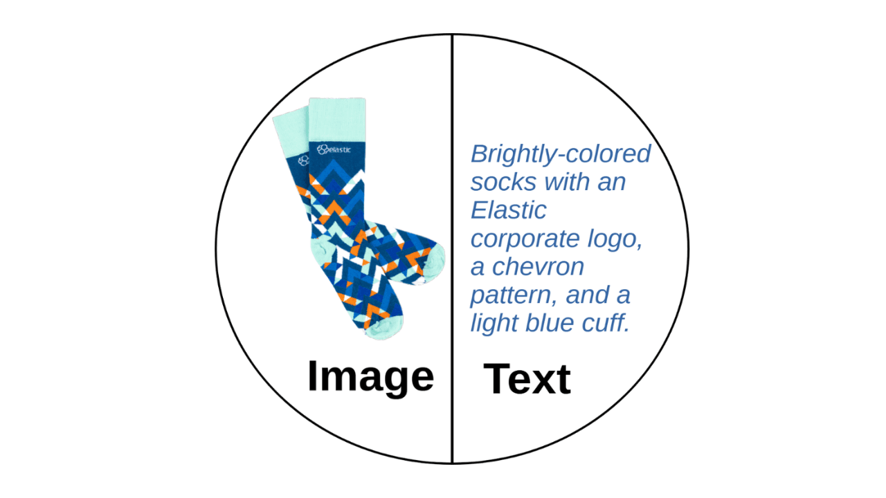
A picture is worth 1.5x the words: What we learned benchmarking product search embeddings
We benchmarked two embedding models on 5,000 real products and found that combining image and text beats either alone by up to 50%. Here's the data and the model that won.
2026年7月13日
The disk that never woke up: what actually decided our Qdrant vector search benchmark rematch
On the same hardware, Elasticsearch and Qdrant land in the same range at 56 QPS. The io_uring disk scorer and memory claims turned out to be the two things that mattered least.

2026年7月21日
4 NVIDIA AI tasks, 1 Elasticsearch API: Embeddings, chat, completion, and rerank
Set up NVIDIA hosted models in Elasticsearch with one API key and a model ID. No custom integration code needed.
2026年7月10日
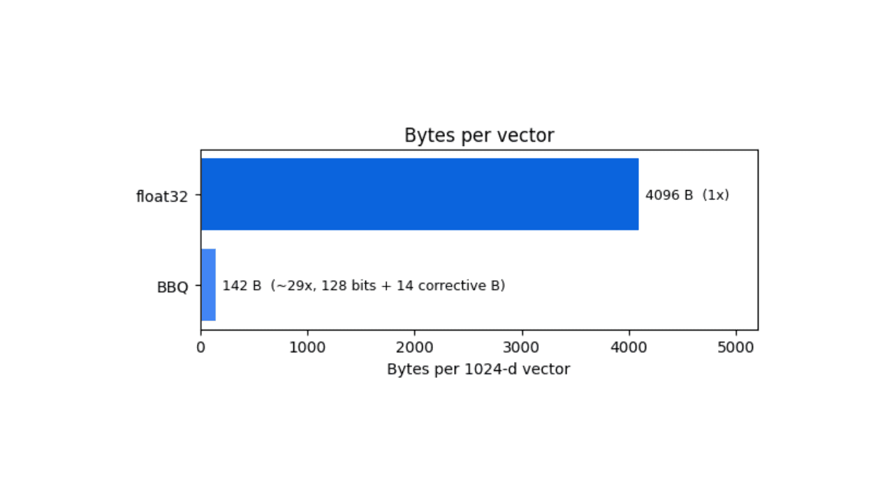
How BBQ shrinks Jina v5 embeddings by 29x without losing recall in Elasticsearch
A hands-on test comparing BBQ and float32 vector indices in Elasticsearch, measuring memory, disk and recall@10 across five languages.
2026年7月7日
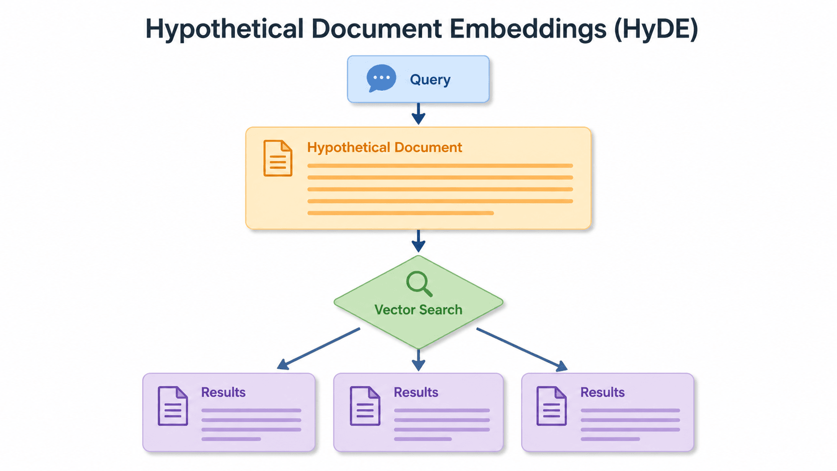
Short queries, formal documents: how HyDE improved semantic search precision by 50% in Elasticsearch
HyDE boosts semantic search precision and recall by 50% on short queries. Here's how to implement it in Elasticsearch with the Inference API and semantic_text.