ベクターサーチはクエリから始まりますが、もしクエリがなければどうすればよいのでしょうか?
組織は大量のドキュメントコレクション(サポートチケット、法的書類、ニュースフィード、研究論文など)を蓄積しており、適切な質問をする前にその内容を理解する必要があります。ラベルやトレーニングデータがなければ、何千もの文書を手動で確認するのは非現実的です。何を検索すればいいかわからない場合、従来の検索は役に立ちません。
この投稿では、この検索の問題に対処するElasticsearchネイティブのアプローチによる教師なし文書クラスタリングと時間軸に沿ったストーリー追跡について説明します。最終的には、次のようにストーリーの文脈を日々にわたってたどることができるようになります。
読み取れる内容:
- なぜクラスタリング埋め込み(検索埋め込みではない)が、クエリーなしでトピック発見を行いたい場合に重要なのか。
- Elasticsearchのk-nearest-neighbor(kNN)とバッチ処理
msearchを使用したトピックにより、密度探査型重心分類で文書をグループ化する方法。 significant_textがクラスターに自動ラベルを付けることで、モデルをトレーニングしなくてもテーマを読めるようにする方法。- テーマが日々どのように変化するかを示す上で、時間軸に沿ったストーリーチェーンが日々のクラスターをどのように結び付けるのか。
この記事は、実行可能なJupyter Notebookから生成されています。全体で見られるインライン出力は、パイプラインからの実際の成果です。付属するノートブックのクローンを作成して、自分で実行してください。
このパイプラインでは、2025年2月のBBCニュースとガーディアンの記事を約8,500件、テストコーパスとして使用しています。ニュースは明確な時間的推移を示すため便利ですが、このパターンは文書の発見が重要なあらゆる場面に適用されます:法的レビュー、コンプライアンスの監視、研究の統合、カスタマーサポートのトリアージ。
スタック:
- Jina v5のクラスタリング埋め込み:トピックグループ化のためのタスク固有の低ランク適応(LoRA)アダプター。JinaはElasticに統合され、そのモデルはElastic Inference Service(EIS)を通じてネイティブで利用可能です。
- Elasticsearch:拡張性のあるkNN、
significant_textラベリング、ベクトルストレージ。 - DiskBBQ:ディスクベースのベクトルインデックス形式で、 Better Binary Quantization(BBQ)と階層的なk-平均法による分割を組み合わせ、近似最近近接傍(ANN)加速を実現します。このインデックス分割はベクトル探索の内部で行われ、本投稿で用いる密度探査型クラスタリング・アルゴリズムとは別です。
bbq_diskはディスクに量子化されたベクトルを格納し、ヒープにはパーティションメタデータのみを保持することで、bbq_hnswと比較してリソース要件を大幅に削減しながら、高い再現率を維持します。 - グローバルクラスタリング + 日々の時間軸に沿ったリンク付け:発見とストーリーの進化。
以下が必要です:
- Elasticsearchの導入(Elastic Cloud、Elasticsearchサーバーレス、またはElastic Self-Managed 8.18+/9.0+):
bbq_disk8.18以降が必要です。オプションのdiversify retrieverセクションは9.3+またはサーバーレスが必要です。 - Jina APIキー:無料プランには1000万トークンが含まれており、これはコアクラスタリング・パイプライン(約425万トークン)をカバーします。オプションの検索対クラスタリング比較は、2番目の埋め込みパスを使用します。
- Guardian APIキー(無料)。
セットアップ
必要なパッケージをインストールしてください:
オプション(このリポジトリからスクレイピングヘルパーを実行する場合のみ):
次に、プロジェクトのルートにある.envファイルでAPIキーを設定します。
このノートブックは load_dotenv(override=True)を呼び出し、局所的な .env 値が優先されます。
パート1:ディスカバリークラスタリング - なぜ埋め込みをクラスタリングするのか?
ほとんどのベクター検索は、クエリを関連文書に一致させるようにトレーニングされた検索埋め込みを使用します 。これは検索には最適ですが、発見には適していません。まったくクエリーせずにコーパスに存在するトピックを見つけたい場合は、類似した文書をグループ化する埋め込みが必要です。
Jina v5では、タスク固有の低ランク適応(LoRA)アダプタを使用してこの問題を解決します。LoRAは、ほとんどのベースモデルの重みを凍結したまま、ターゲットとなる内部層に小さな低ランクの更新を加えるため、完全な再トレーニングを行うことなく、モデルの挙動が特定のタスクにシフトします。同じベースモデルでも、taskパラメータによって異なる埋め込みが生成されます。
| タスク | 訓練の目的 | ユースケース |
|---|---|---|
| retrieval.passage | クエリーと文書のマッチング | Search、Retrieval-Augmented Generation(RAG) |
| クラスタリング | トピックのグループ化(密度が高いクラスタリングの最適化) | 発見、分類 |
クラスタリング・アダプターは、同じトピックに関する文書を埋め込み空間で近づけ、異なるトピックに関する文書を離すように訓練されています。下のビジュアル比較で、その違いが具体的にわかります。
検索とクラスタリング:視覚的な比較
違いを確認するために、両方のタスクタイプを含むサンプル文書を埋め込んでいます。クラスタリングは元の1024次元の埋め込み空間で実行されます。均一多様体近似と射影(UMAP)は、可視化のためそれらの埋め込みを2Dに投影する目的でのみ使用されます。東映UMAPは局所的な近傍構造を保持するため、クラスターの分離を比較する上で有用です。
以下では、同じ480件の文書のサンプルが両方のタスクタイプに埋め込まれ、UMAPで2Dに投影されています。クラスタリングパネルで、より密集していて、分離された色群を探します。
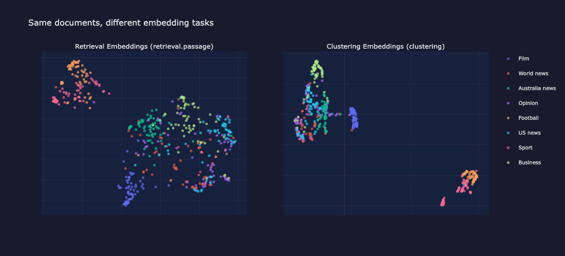
検索埋め込み(左)はトピックを広く分散させます。クラスタリング埋め込み(右)は、同じドキュメントからより緊密で分離されたグループを生成します。
クラスタリング埋め込みは、より緊密で視覚的に際立ったグループを生み出します。検索用の埋め込みはトピックをより均等に分散させ、(きめの細かい類似性で)検索する上で理想的です。しかし、発見のためには、緊密なトピッククラスターが重要です。
このため、このチュートリアルの残りの部分では task="clustering" が使用されています。
データセットの読み込み
次のコーパスは、2025年2月の2つのニュースソースを組み合わせています。
- RealTimeData/bbc_news_alltime HuggingFaceデータセット経由のBBCニュース。
- Guardian Open Platform API経由のThe Guardian。
複数のソースがあると、クラスタリングがトピックではなくソース固有のスタイルを見つけることを検証するのに役立ちます。
クラスタリングタスクによる埋め込み
Jina v5 APIはすべての文書に対してtask="clustering"で呼び出されます。埋め込みはディスクにキャッシュされるため、その後の実行ではAPIを完全にスキップします。
API呼び出しはシンプルです。taskパラメータが、典型的な埋め込み使用との主な違いです。
以下のタイミングはキャッシュヒットを反映しています。APIに対する最初の実行は、コーパスサイズによって時間がかかります。
単一のElasticsearchインデックスへのインデキシング
発見クラスタリングでは、1か月間を1つのインデックス(docs-clustering-all)にまとめます。日々の分割は、時間軸に沿ったストーリーリンクのために後から行われます。
インデックスマッピングでは、ベクトルフィールドにbbq_diskを使用します。
1024次元のfloat32ベクトルは4KBです。bbq_disk は階層的k-means法を使用してベクトルを小さなクラスターに分割し、それらをバイナリ量子化し、再スコアリングのためにフルプレシジョンのベクトルをディスクに格納します。パーティションのメタデータのみがヒープに存在し、そのため大規模なコーパスでもメモリ要件は低く抑えられます。より多くのヒープを許容できるワークロードの場合、bbq_hnsw は、より高いリソースコストでより高速な検索を行うための階層的ナビゲーシブル・スモールワールド(HNSW)グラフを構築します。
dense_vectorフィールドタイプは複数の量子化戦略をサポートしています:bbq_diskとbbq_hnswは、ここで使用されている1024次元ベクトルのような高次元埋め込みに最適です。
クラスタリング:密度探査型重心分類
HDBSCANのような従来型のクラスタリングアルゴリズムでは、完全なn×dベクトル行列をメモリに保持し、フルパス更新を繰り返し実行できることを前提としています。8,495件のドキュメントを1024次元で扱う場合、処理可能(最大35MB)ではあるものの、このアプローチは追加のインフラストラクチャーなしでは数百万の文書にスケールすることはできません。
このアルゴリズムは、ボロノイ領域への割り当て割り当てとノイズフロアによるKMeans++法の初期化と概念的には似ていますが、ElasticsearchのkNN検索を計算プリミティブとして使用し、ほぼ全ての作業をサーバー側で行います。
- 文書の5%を密度プローブとしてサンプリングします(ランダムサンプル、最低50件)。
- バッチ処理された msearch kNNによるプローブ密度。各プローブはkNNクエリを実行し、隣接プローブの平均類似度を記録します。平均類似度が高い=埋め込み空間の密な領域。
msearchは単一のHTTPコールで複数の検索リクエストを送信し、これは重要です。密度プローブは数百のkNNクエリを生成し、それらをバッチ処理することでリクエストごとのオーバーヘッドを回避します。 - 多様性を考慮した高密度シードの選択:中央値以上の密度を持つ候補は、密度の降順でソートされ、既存のすべてのシードとのコサイン類似度が分離閾値を下回る場合にのみ貪欲に受け入れられます。これがクライアント側での唯一の計算です(8,000件の文書で最大0.01秒)。
msearchkNNで全ての書類を重心に照らして分類します。各シードが重心として機能し、kNN検索は類似度しきい値を超える近接文書を取得します。各文書は、最も高いスコアを返した重心に割り当てられます。小さなクラスターはノイズとして処理されます。
Elasticsearchが面倒な処理を担当します:msearchは密度プローブ、msearchは分類、significant_textはラベル付けを担います。このコーパス(8,495件の文書)では、5%の密度プローブサンプルが425件のkNNプローブクエリを開始し、msearchが9つのHTTPコール(バッチサイズ50)にバッチ処理され、プローブごとに1つのリクエストを処理することによるオーバーヘッドを回避します。bbq_diskANNルックアップと組み合わせることで、クラスタリング段階を高速かつスケーラブルに保つことができます。kNNクエリは、クラスタリングパス中の速度のために最小のnum_candidates値を使用します。本番環境の検索クエリでは、レイテンシを犠牲にしてリコールを向上させるために、より高いnum_candidates値を使用する必要があります。
クラスターは各重心の周りの埋め込み空間の密度によって決定される実際的なサイズを持ち、厳格なkの上限によって決定されるものではありません。密なトピック領域はより大きなクラスターを生み出し、ニッチなトピックは小さなクラスターを生み出します。
KMeansやHDBSCANが実用的ではない理由
KMeans法は球状クラスターを想定しており、メモリに完全なn×d行列が必要です。メモリに収まるコーパスの場合、HDBSCANは強力な代替手段です。任意のクラスタ形状に対応でき、密度に関するセマンティクスも十分に理解されています。
密度探査型重心アプローチは、異なるニッチをターゲットとしています。ストレージ、検索、およびクラスタリングを1つのシステムで行いたい場合や、スケールがクライアント側の行列操作を実用的でなくするようなコーパスです。これは、Elasticsearch kNNを計算プリミティブとして使用し、任意のクラスターサイズを処理し、ほぼすべての計算をサーバー側で行います。
ノイズレートについて理解する
最大28%のノイズ率は設計によるもので、故障モードではありません。設定されたsimilarity_thresholdでどの高密度クラスターにも適合しない文書は、一致率が低いと強制的に判断されるのではなく、割り当てられずに残されます。これは品質ゲートの役割を果たします:意見を記したコラム、短い記事、そして一回限りのストーリーは、一貫したグループを定義する主題の密度が不足しているため、クラスタリングに抵抗する性質があります。
しきい値は調整可能です。similarity_thresholdを下げると、より積極的なクラスタリングが生成されます(より多くの文書が割り当てられますが、クラスターは緩くなります)。一方、これを上げると、クラスターが引き締まり、ノイズの割合が増加します。こうした様々なニュースコンテンツを含むコーパスにおいては、約30%のノイズは妥当な動作基点と言えます。本番環境での導入は、分野固有の品質基準に合わせてしきい値を調整することが推奨されます。
significant_textを使用した自動ラベル付け
各クラスターには人間が読みやすいラベルが必要です。Elasticsearchのsignificant_textアグリゲーションは、フォアグラウンドセット(クラスター)とバックグラウンドセット(完全なコーパス)を比較して、異常に頻繁に現れる用語を見つけます。
内部的には、絶対頻度の変動と相対頻度の変動のバランスを取る統計的ヒューリスティック(デフォルトではJLHスコア)を使用しており、機械学習や大規模言語モデル(LLM)の呼び出しは行っていません。英国の政治に関するクラスターでは、starmer、labour、downingのような用語が浮かび上がる可能性があります。これらの用語は、全体的なニュースコーパスと比較して、そのクラスターで不釣り合いに頻出しているためです。
このグローバルパスでは、ラベルはdocs-clustering-allに対して直接計算されるため、前景と背景の両方が月全体のデータから描画されます。パート2では、ラベル付けに日次インデックスパターン(docs-clustering-*)を使用します。これは、クエリで一致するすべてのインデックスを同時に対象にできるワイルドカードで、significant_textにより広い背景を与えてコントラストを高めます。
最小クエリー形状は次のようになります。
significant_text また、品質ゲートの役割も果たします。有意な用語を生成しないクラスターには、特徴的な語彙がありません。これらはまとまりのないグループであり、誤解を招くようなラベルを付けるのではなく、ノイズとして分解する必要があります。
軽量で決定論的なクリーンアップステップで、ノイズの多いラベルの用語(数値トークン、一般的な単語)を削除し、必要に応じて代表的な見出しに切り替えます。これにより、ラベルをElasticsearchネイティブのまま維持しつつ、可読性を向上させます。
クラスターの可視化
以下の可視化は、グローバルクラスタリングパスが発見した内容を示しています:クラスター化された文書とノイズ文書の日付ごとの内訳、全月のUMAP投影、およびクラスターがソースではなくトピックを反映していることを確認するソースミックスチャート。
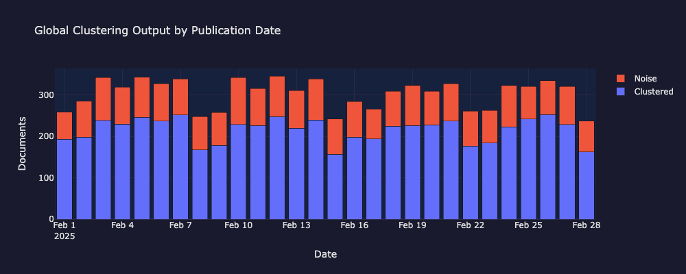
2025年2月におけるクラスター化された文書とノイズ文書の日次分布。
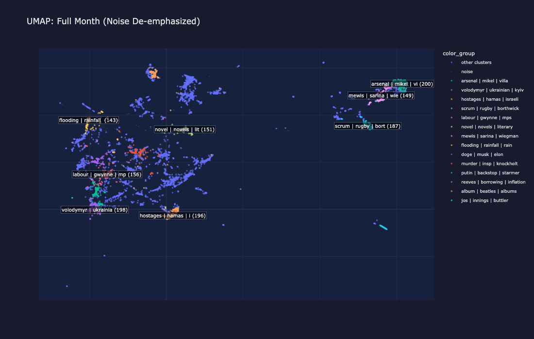
1か月間のUMAP投影:各色の島はトピッククラスター、灰色の点はノイズを表す
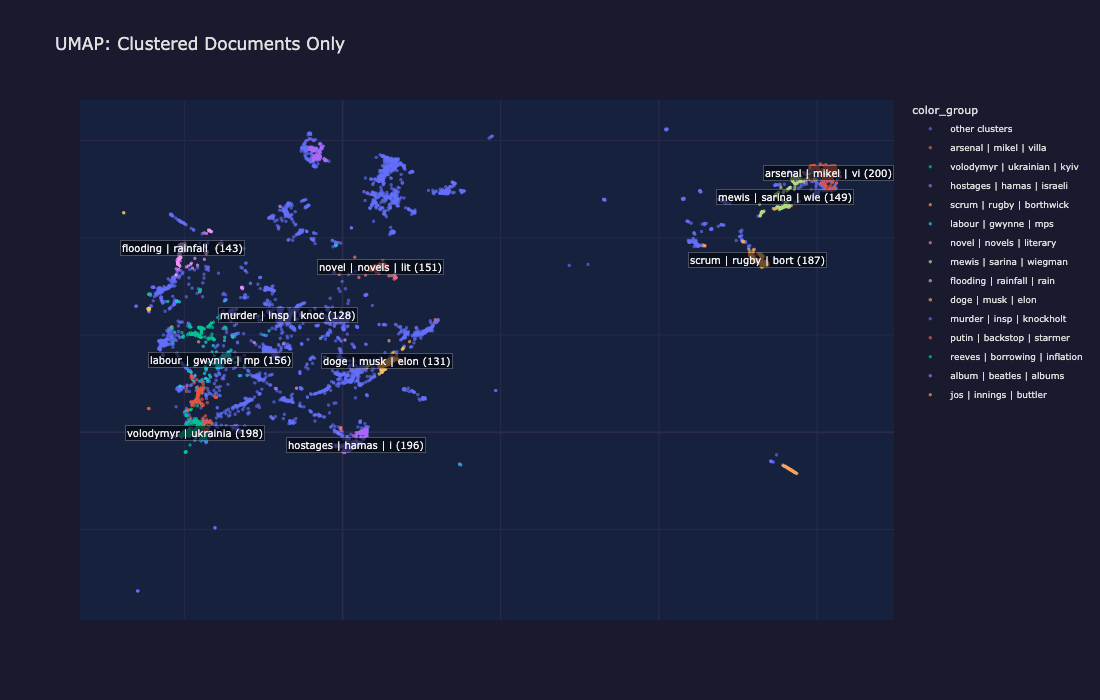
クラスター化された文書のみ:ノイズを除去することで、主題構造がより明確に明らかになる
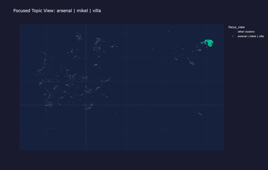
一つのクラスター(プレミアリーグサッカー)を他のすべてのクラスターと比べて強調するフォーカスビュー。
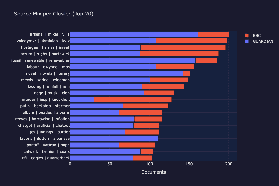
クラスターごとのソース混合:BBCとガーディアンの両方がすべての主要なクラスターに現れ、ソースベースのグループ化ではなくトピックベースのグループ化が確認できます。
UMAPの色のついた島はそれぞれがクラスターを表しています。クラスターは、純粋に類似性を埋め込むことで発見された、同じトピックに関する記事の集合です。灰色のノイズポイントは、いずれのクラスターにもきれいに収まらなかった記事(多くの場合、短い記事、意見記事、または一回限りのストーリー)です。
情報源の内訳図を見ると、各クラスターにはBBCニュースとガーディアンの両方からの記事が含まれていることが確認できます。クラスタリングは、ソースではなくトピックを見つけ出すものであり、まさに教師なし学習から期待される結果です。
Diversify Retrieverによるクラスター幅の調査
通常のkNNは、クラスターの重心(密なコア)に最も類似した文書を返します。しかし、実際のクラスターはサブトピックも対象にします。The Diversify Retrieverは、Maximal Marginal Relevance(MMR) を使用して、重心に関連するだけでなく、互いに異なる文書を抽出します。
鍵となるパラメータは λ(ラムダ)です。
- λ = 1.0 → 純粋な関連性(通常のkNNと同じ)。
- λ = 0.0 → 純粋多様性(最大限に分散された結果)。
- λ = 0.5 → バランスが取れている:トピックに関連しているが、異なる角度をカバーしている。
バージョン注記:Diversify RetrieverはElastic Cloud ServerlessおよびSelf-Managed Elasticsearch 9.3+で利用可能です。以前のバージョンでも、クラスタリングと時間軸に沿ったリンク付けのセクションに従うことができます。この探索ステップのみ、Diversify Retrieverが必要です。
最小Retrieverリクエストの形状は次のようになります。
type、field、および query_vector パラメーターは、diversifyレベルで必要です。field はMMRに結果間の類似性に使用する dense_vector フィールドを指示し、query_vector は関連性スコアリングの参照点を提供します。
これにより、単に「その中心は何か?」という問いではなく、「このクラスターは実際に何を対象としているのか?」という問いに答えることができます。
プレーンなkNNは、トピックの1つの角度、つまり中心点および互いに最も類似したドキュメントの周りにクラスターを形成します。Diversify Retrieverは、同じクラスターの異なるファセット、つまりサブトピック、異なるソース、多様な視点を提示します。
多様性指標はこれを定量的に裏付けます。Diversify Retrieverの結果では、平均ペアワイズ類似度が低く、これは返された文書がより広範囲をカバーしていることを意味します。
これは以下の用途に役立ちます。
- クラスターが実際に対象としている内容を理解。その中心だけでなく端も含め理解します。
- 要約の生成。多様で代表的な文書は、LLMにより良い材料を提供します。
- 人によるレビューや下流工程でのラベリングのために、代表的な例を発見。
- 品質チェック。多様な結果が一貫性に欠けている場合、クラスターの分割が必要かもしれません。
パート2:時間軸に沿ったストーリーチェーン
日をまたいだデータストーリーの追跡
パート1では、トピック発見のために1か月全体をグローバルにクラスタリングしました。時間軸に沿ったフローでは、同じ密度プローブの重心分類が日次インデックスごとに1日単位で独立して実行され、その後、クラスターが隣接する日々にわたってリンクされます。注意:日々のクラスターはパート1のグローバルクラスターとは独立しており、それぞれの1日はその日のコンテンツに合わせて独自のクラスター割り当てとラベルを生成します。
関連付けの手法:サンプルとクエリ
A日目の各クラスターについて:
- いくつかの代表的な文書をサンプルとして選択します。
- kNNをB日目のインデックスに対して実行します。
- B日目のクラスターごとにヒット数を数えます。
- ヒット率がしきい値(kNNの割合≥ 0.4)を超える場合は、リンクを記録します。
この処理は高速で(クラスターごとにわずかなドキュメントのみがクエリされ、すべてではありません)、ElasticsearchのネイティブkNNを使用し、外部ツールは必要ありません。
kNN分数が100%ということは、ソースクラスターからサンプリングされたすべてのドキュメントが同じターゲットクラスターに到達していることを意味し、これは異なる日付間のリンクが理論上最も強くなります。ほとんどの上のリンクはフットボール関連で、これは理にかなっています。プレミアリーグは毎日報道され、高いトピックの一貫性があります。
The score | operator | gedling → league | striker | season リンクは、ニッチなローカルフットボールクラスター(Gedling はノンリーグクラブです)が翌日に広範なプレミアリーグクラスターに吸収される例であり、これは異なる粒度での日々の再クラスタリングの自然な効果です。
ストーリーチェーンの構築
ストーリーチェーンとは、連日にわたって連続した一連のクラスターです。
個々のペアワイズリンクは、月曜日の「UK politics」クラスターが火曜日のクラスターにリンクしていることを示しています。チェーンはストーリー全体を明らかにします。月曜日に始まり、週を通して展開し、金曜日までに消えていくストーリーです。
チェーンは、kNN分数が0.4以上のリンクから貪欲に構築されます。これは、ソースクラスターからサンプリングされたドキュメントの少なくとも40%が単一のターゲットクラスターに到達したことを意味します。最も古いクラスターから開始し、アルゴリズムは常に最も強い発信リンクを追跡します。
最も長いチェーンは、ウクライナとロシアに関する報道を19日間連続で追跡していますが、2025年2月の地政学的な緊張が持続していることを考えると、これは驚くべきことではありません。2番目に長いチェーンは、19日間にわたるプレミアリーグのサッカーを追跡するものです。より短いチェーンは、映画賞シーズン(6日間)、シックス・ネーションズラグビー(10日間)、英国の政治指導者に関する報道(7日間)を追跡しています。それぞれのチェーンは、アルゴリズムが日々のインデックス全体にわたる埋め込み類似性のみから発見したストーリー展開を表しています。
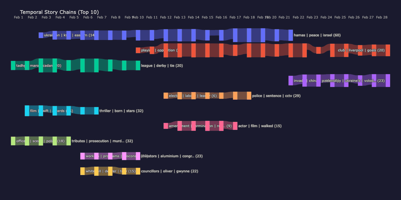
サンキー:ストーリーの流れを可視化する
サンキーダイアグラムは、リンクの幅がつながりの強さを表す流れの可視化です。ここでは、各垂直バンドが1日を表し、各ノードは日々のクラスター(ドキュメント数によってサイズが決まる)であり、各色のパスは時間の経過に沿って1つのストーリーチェーンを追跡します。リンク幅はkNNのオーバーラップ強度をエンコードします。リンクが太いほど、サンプリングされたドキュメントの数がより多くターゲットクラスターに到達したことになります。色はチェーンごとに分かれているので、左から右へ流れる1つのカラーパスで1つのストーリーの進行がわかります。
たとえば、ウクライナとロシアのチェーン(比較的長い経路の一つとして示されている)は、2月初旬から第3週まで途切れることなく続いており、一貫して太い線で結ばれていることから、日々の話題の連続性が強いことがわかります。
2025年2月に流れる時間軸に沿ったストーリーチェーン各色のパスは、複数日にわたって続くストーリーを表し、リンクの幅はkNNの重なりの強さを示します。
このアプローチがもたらすメリット
このウォークスルーでは、Elasticsearch上に構築された完全な教師なしドキュメントクラスタリング・パイプラインについて説明しました。
- クラスタリング埋め込み:Jina v5のタスク固有のアダプターは、トピックのグループ化に最適化された埋め込みを生成し、単なるクエリと文書のマッチングだけではありません。
- グローバルな発見クラスタリング:1つのインデックスで1か月間をクラスタリングすることで、日をまたいだトピックの発見を最大化します。
- 密度プローブによる重心分類:5%をサンプリングし、
msearchkNNを介して密度をプローブし、多様な高密度シードを選択し、すべての文書を重心に対して分類します。Elasticsearchは負荷の高い計算を処理します。シード選択のみがクライアント側で実行されます(最大0.01秒)。 significant_textラベリング:有意性テストは、MLモデルや手動アノテーションなしで意味のあるクラスタラベルを生成します。有意な項を生み出さないクラスタは非整合となり、ノイズに格下げされます。これは内蔵された品質ゲートです。- 時間軸に沿ったストーリーのリンク付け:日次インデックスとサンプルおよびクエリのクロスインデックスkNNは、ストーリーが時間とともにどのように進化するかを追跡します。
重要なポイント
- 埋め込みタスクの種類が重要です。クラスタリング埋め込みは、測定可能かつより緊密な話題のグループを生成します。
- Elasticsearchはストレージ層およびクラスタリングエンジンの両方としてkNN検索を通じて機能します。
- 密度探査型重心分類は、ほぼすべての計算をサーバー側で行い、埋め込み空間の密度によって決定される合理的なサイズのクラスターを生成します。
significant_text高速で解釈可能で、自動ラベリングと品質管理の両方に効果的です。
このアプローチは、以下の場合に有用です。
- タイムスタンプ付きのテキストがあり、ラベル付きトレーニングデータを使用せずにトピックを発見したい場合があります。
- ストレージ、ベクトル検索、ラベル付け、および時間軸に沿ったリンク付けのために、1つのスタックが必要な場合があります。
検討すべき拡張機能:
- 複数期間クラスタリング(週間、月間集計)。
- リアルタイムのインジェストと段階的なクラスター割り当て。
- LLM生成のクラスタサマリーは、significant_text項をシードとして用います。
- より大規模なスケールでは、サンプリングされたKMeansの重心が密度ベースのクラスタリングのウォームスタートシードとして機能し、探査フェーズのコストを削減できます。
はじめましょう
タイムスタンプ付きの文書コーパスを差し替えます。日付のあるテキストのコレクションであれば、このパイプラインで利用可能です。完全なノートブックとサポートコードは、付属レポジトリで入手できます。
- Elastic Cloudの無料トライアルを開始:
bbq_diskサポート付きのマネージドクラスターを数分でご利用いただけます。 - Elasticsearch Serverlessをお試しください:クラスターの管理は不要で、自動的にスケールし、このウォークスルーのすべてをサポートします。
関連記事
2026年4月23日
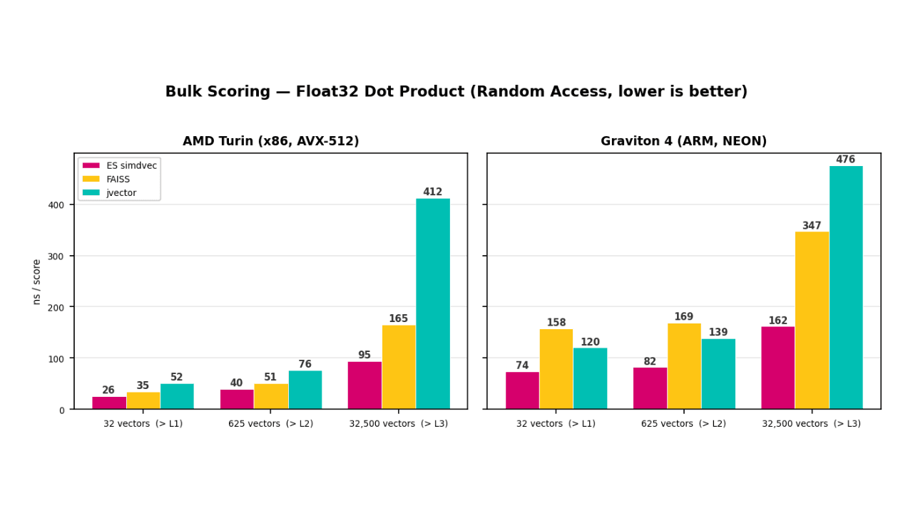
ベクトル検索を世界最速のものにするためにElasticsearch simdvecを構築した方法
Elasticsearchのすべてのベクトル検索クエリの基盤となる、手作業で調整されたSIMDカーネルライブラリElasticsearch simdvecの構築方法。
2026年5月4日
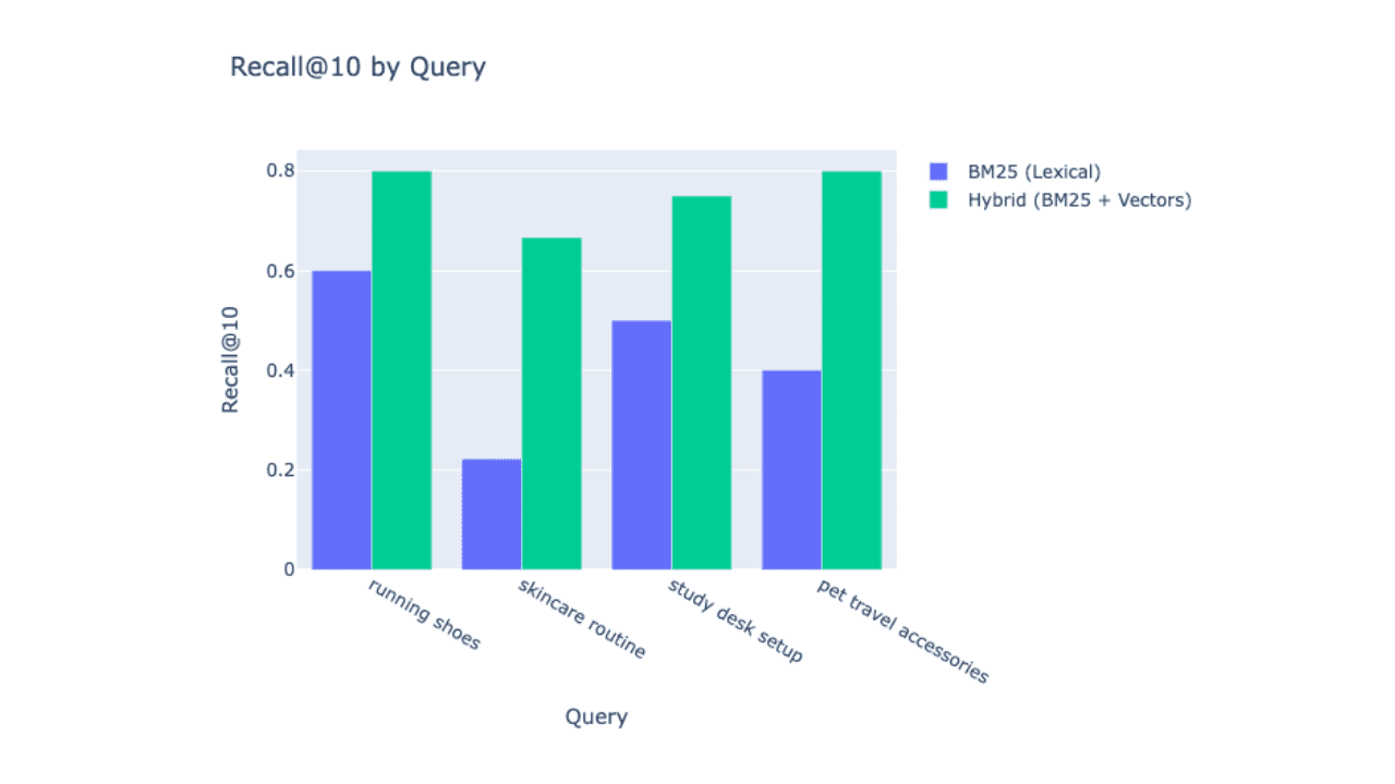
Elasticsearchの検索再現率を測定・改善する方法:ハイブリッド検索で0.43から0.75へ
Elasticsearchにおける検索再現率を測定および改善する方法を学びましょう。BM25の語彙検索とJina AIのベクトル埋め込みを組み合わせ、rank_eval APIを使用して実際の数値で改善効果を検証します。

2026年4月2日
TSDSとILMが出会うとき:遅延データを拒否しない時系列データストリームの設計
TSDSの時間制限はILMフェーズとどのように相互作用するのか、そして遅れて到着するメトリクスを許容するポリシーを設計する方法。
2026年4月1日
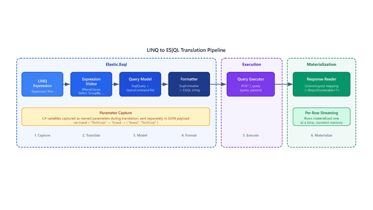
LINQ to Elasticsearch ES|QL:C#を記述してElasticsearchをクエリ
Elasticsearch .NETクライアントに新しく追加されたLINQ to Elasticsearch ES|QLプロバイダをご紹介します。C#コードを自動的にES|QLクエリに変換できます。
