誰もがベクトル検索が瞬時に行われることを望んでいますが、高次元ベクトルではデータ量が膨大になります。1,024次元のfloat-32ベクトルは1つのメモリを大量に消費し、他の何百万ものベクトルと比較すると計算量が多くなります。
これを解決するために、Elasticsearchのような検索エンジンは主に2つの最適化戦略を使用します。
- 近似検索(Hierarchical Navigable Small World [HNSW]):すべての文書をスキャンする代わりに、ナビゲーショングラフを構築して、回答の可能性が高い近傍に素早くジャンプします。
- 量子化:メモリ使用量を削減し、計算速度を向上させるために、ベクトルを圧縮します(例えば、32ビット浮動小数点数から8ビット整数、あるいは1ビットのバイナリ値へ)。
しかし、最適化にはしばしば精度という代償が伴います。
「データを圧縮し、検索中にショートカットを取ると、最高の結果を見逃すのではないか?」「この最適化は検索エンジンの関連性を低下させるのではないか?」といった恐れは正当です。
Elasticの量子化が結果を低下させないことを証明するために、DBpedia-14 データセットを使用して再現可能なテストハーネスを構築し、Elasticsearchのデフォルトの最適化を使用する際に、速度と引き換えにどれだけの精度(具体的には再現率)を犠牲にしているかを正確に計算しました。
要約すると、それはおそらく想定よりもずっと少ないでしょう。こちらのノートブックをチェックして、ぜひご自身でお試しください。
定義(非専門家向け)
コードを見る前に、いくつかの用語について確認しておきましょう。
- 関連性対再現率:関連性 は主観的で(良いものが見つかったか?)、再現率は数学的なものです。データベース内にクエリと完全に一致する文書が10件あり、検索エンジンがそのうち9件を見つけた場合、再現率は90%(または0.9)です。
- 完全一致検索(フラット):総当たり法とも呼ばれ、検索エンジンはインデックス内のすべての文書をスキャンし、距離を計算します。
- 長所:100%完璧な再現率。
- 短所:計算コストが高く、スケール時の処理速度が遅くなる。
- 近似探索(HNSW):いわゆる「ショートカット」の方法。検索エンジンは HNSW グラフを作成し、グラフを巡回して最も近い隣接点を探します。
- 長所:非常に高速で拡張性が高い。
- 短所:グラフの探索が早すぎて停止すると、近傍を見逃す可能性がある。
実験:完全一致と近似探索の比較
再現率をテストするために、テキスト分類モデルのトレーニングと評価によく使用される、14のオントロジークラスにわたるタイトルと要約の大規模なデータセットDBPedia-14データセットを使用しました。具体的には、「Film」カテゴリに焦点を当てます。最適化された生産設定を、数学的に完璧な真値と比較したいと考えました。
この実験では、テキスト表現の業界ベンチマークをリードする最先端の多言語モデルjina-embeddings-v5-text-smallモデルを使用しています。このモデルを選んだ理由は、高性能埋め込みの現在の標準となっているためです。Jina v5の優れた精度とElasticsearchのネイティブ量子化を組み合わせることで、計算効率が高く、検索品質にも妥協のない検索アーキテクチャを実証できます。
二重マッピングを使用したインデックスを設定し、同じテキストを同時に2つの異なるフィールドに取り込みました。
content.raw(タイプ:flat)。これにより、ElasticsearchはFloat32ベクトル全体の総当たりスキャンを実行することになります。これにより完全一致の結果が返され、ベースラインとして使用されます。content(タイプ:semantic_text)。デフォルトではHNSW + Better Binary Quantization(BBQ)を使用しています。これは、近似一致のための標準的かつ最適化された生産設定です。
Recall@10 テスト
指標としては、Recall@10を使用しました。
50本のランダムな映画を選び、両方のフィールドに同じクエリを実行しました。
- 完全一致(フラット)検索で上位10個の近傍が ID [1, 2, 3... 10] であると示されている場合。
- また、近似(HNSW)検索では、ID [1, 2, 3... 9, 99] が返されます。
- 上位10位のうち、9位を正しく特定できました。スコアは0.9です。
こちらが使用したマッピングです。
結果:成功の「横ばい線」
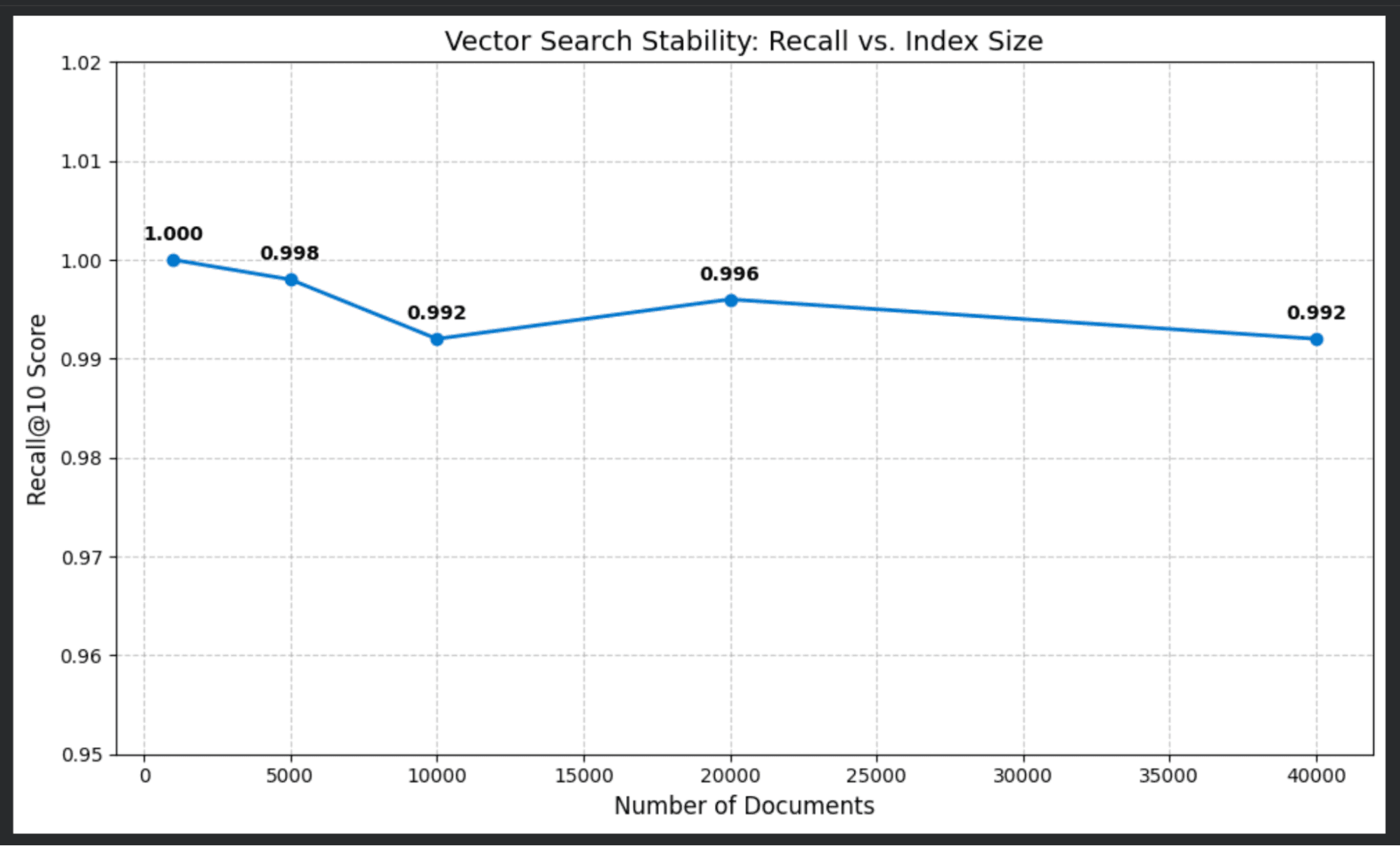
スケールテストを実行し、完全なデータセットを再読み込みし、1,000~40,000件の文書のインデックスサイズに対してテストしました。
再現率スコアに何が起こったかは以下のとおりです。
| ドキュメント | Recall@10スコア |
|---|---|
| 1,000 | 1.000 (100%) |
| 5,000 | 0.998 (100%) |
| 10,000 | 0.992 (99.4%) |
| 20,000 | 0.999 (99.0%) |
| 40,000 | 0.992 (98.8%) |
結果は驚くほど安定していました。スケールアップしても、近似検索は総当たりの完全一致検索と99%超の確率で一致しました。
なぜこれほど上手くいったでしょう?
ベクトルをバイナリ値に圧縮すると、これよりも精度が低下すると考えられるかもしれません。その理由は、Elasticsearchが検索を処理する方法にあります。
今日のほとんどの埋め込みモデルは、大きなFloat32ベクトルを出力します。探索を効率的にするために、Elasticsearchは高次元ベクトルに対して量子化を使用します。具体的には、バージョン9.2以降、デフォルトでBBQを使用するようになりました。
BBQは再スコアリングメカニズムを採用しています。
- トラバーサル:検索エンジンは圧縮された(量子化された)ベクトルを使ってHNSWグラフを高速に走査します。ベクトルが小さいため、効率的にオーバーサンプリングを行い、パフォーマンスを損なうことなく、より多くの候補リスト(例えば、類似性の高い上位100件の文書)を収集できます。
- 再スコアリング:候補が見つかったら、その数件の文書について完全精度の値を取得して、最終的な正確なランキングを計算します。
これにより、量子化による高速な処理と、最終的なソートにおける浮動小数点数の精度という、両方の利点を享受できます。
もっと良くできるでしょうか?
注目すべき点は、ここで確認している結果がデフォルト設定とデータのランダムサンプリングを使用していることです。これは高性能の出発点とお考えください。Jina v5は非常に優れていますが、これらの再現率スコアはすべてのデータセットに対して「万能な」保証ではありません。すべてのデータ収集には独自の特性があり、さらにパフォーマンスを向上させるために調整することは可能ですが、常に自分の特定のデータに対してベンチマーク設定を行い、どこまで性能を引き出せるかを確認する必要があります。
まとめ
これは非常に小規模なテストです。ただし、この演習の目的は埋め込みモデルやBBQを個別に測定することではありません。最小限のセットアップで、データセットの再現率を簡単に測定する方法を示すことです。
このテストを独自のデータで実行したい場合は、こちらのノートブックをチェックして試してみてください。
関連記事
2026年4月23日
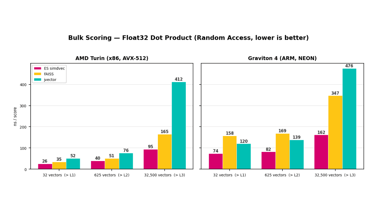
ベクトル検索を世界最速のものにするためにElasticsearch simdvecを構築した方法
Elasticsearchのすべてのベクトル検索クエリの基盤となる、手作業で調整されたSIMDカーネルライブラリElasticsearch simdvecの構築方法。
2026年5月4日
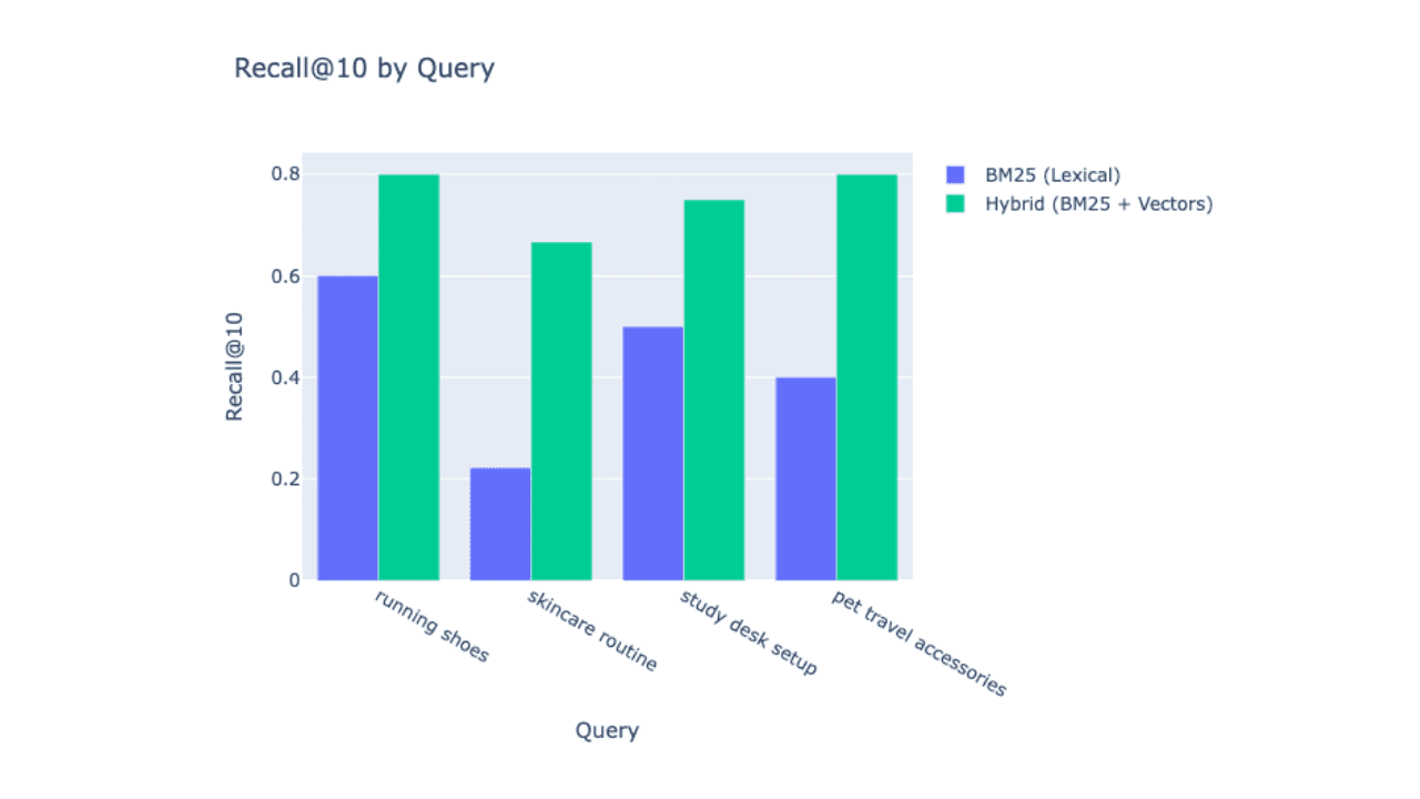
Elasticsearchの検索再現率を測定・改善する方法:ハイブリッド検索で0.43から0.75へ
Elasticsearchにおける検索再現率を測定および改善する方法を学びましょう。BM25の語彙検索とJina AIのベクトル埋め込みを組み合わせ、rank_eval APIを使用して実際の数値で改善効果を検証します。
2026年4月10日
Elasticsearch + Jina埋め込みによる教師なし文書クラスタリング
ElasticsearchとJina埋め込みを使用した教師なし文書クラスタリングへの実用的で再現可能なアプローチ。

2026年4月2日
TSDSとILMが出会うとき:遅延データを拒否しない時系列データストリームの設計
TSDSの時間制限はILMフェーズとどのように相互作用するのか、そして遅れて到着するメトリクスを許容するポリシーを設計する方法。
2026年4月1日
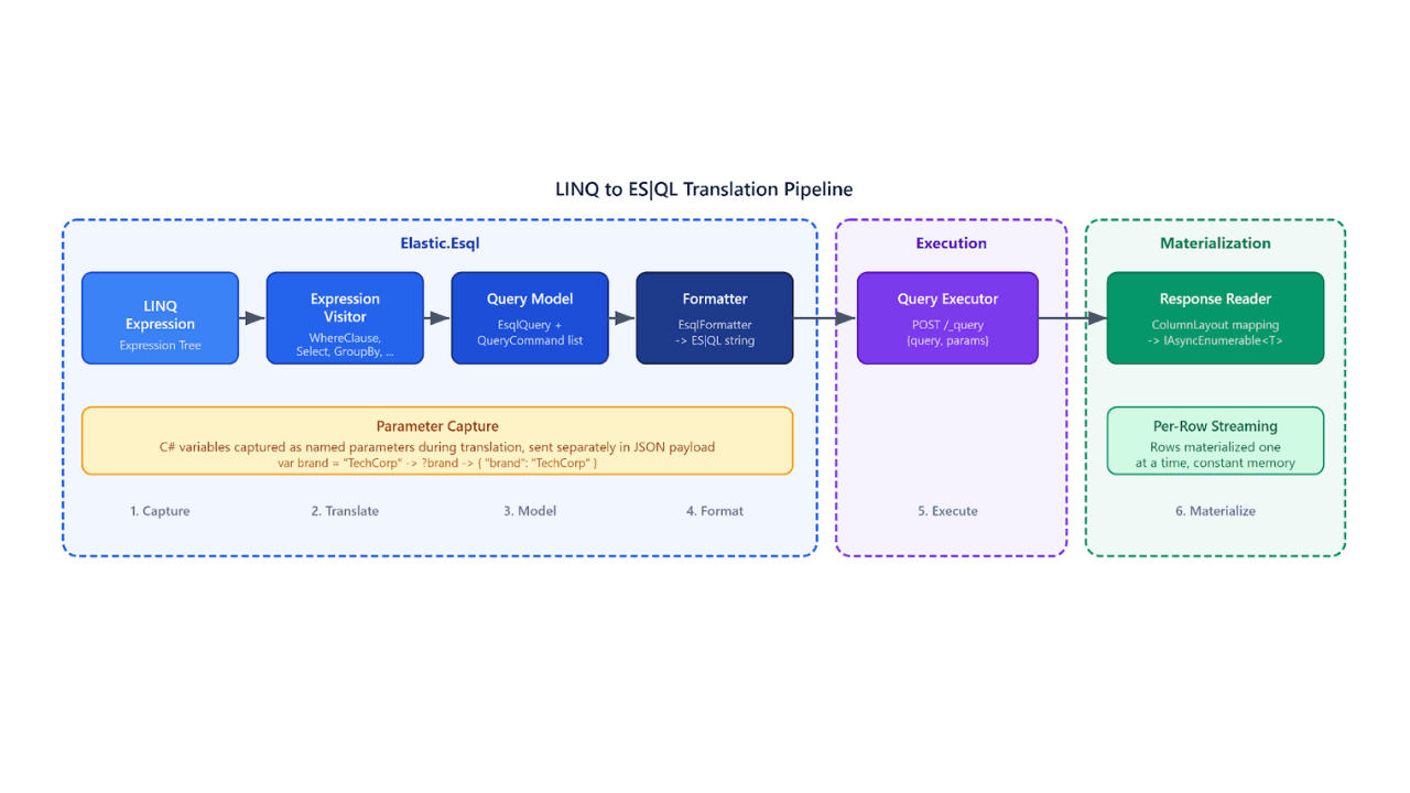
LINQ to Elasticsearch ES|QL:C#を記述してElasticsearchをクエリ
Elasticsearch .NETクライアントに新しく追加されたLINQ to Elasticsearch ES|QLプロバイダをご紹介します。C#コードを自動的にES|QLクエリに変換できます。