Changes to Elastic Machine Learning Anomaly Scoring in 6.5
In a previous blog post about anomaly scoring, we explained in depth how Elastic machine learning scores and reports anomalies in different ways. In this blog, we discuss two new major changes introduced in version 6.5 that affect how anomaly scores are determined. These changes are with respect to the normalization of partitions and anomalies that occur across multiple time buckets.
Normalization of Partitions
As mentioned in our previous blog, normalization is the mechanism by which raw anomaly probabilities are mapped to more actionable values in the range 0 - 100. What wasn’t mentioned, however, were the details around how the normalization process works when the job is split (like in a “multi-metric” job or when using partition_field_name in an “advanced” job) as the means to create many simultaneous analyses.
The presence of partitions does indeed make independent statistical models for each partition - that has been always the case. However, a common misconception was that each partition’s normalized anomaly scores were also completely independent — this was not true. The normalized scores of anomalies took into consideration the full range of probability values of all anomalies across all partitions in the job. As a result, users were surprised to see relatively low scores for seemingly “big” anomalies occurring in certain partitions. This was because more egregious anomalies were occurring (or had recently occurred) in other partitions, thus taking ownership of the higher normalized scores.
To help illustrate the challenges that users were seeing before 6.5, an example is shown below, where a single time series (airline:COX) was analyzed in isolation in a single-metric job:
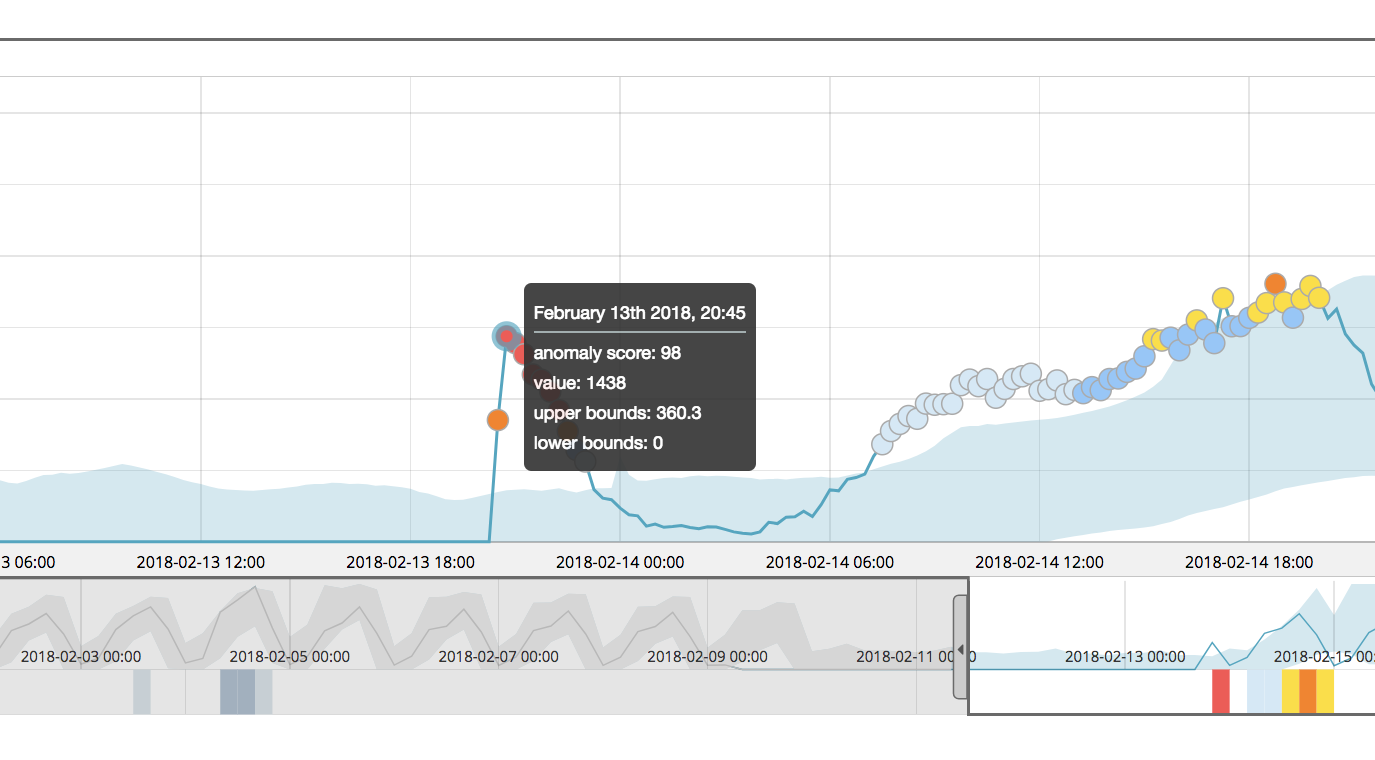
The highlighted anomaly is critical, with a normalized anomaly score of 98. This intuitively seems reasonable, given the apparent magnitude of the change in behavior at this point in time.
But when this time series was analyzed as part of a multi-metric job with many other partitions (split on airline), the results for this airline:COX partition are markedly different:
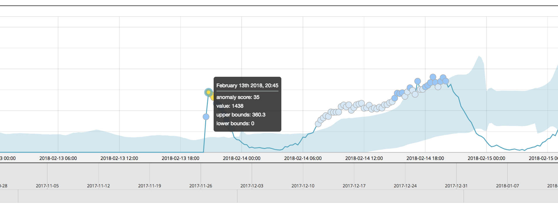
In this case, the same anomalous event had been assigned a normalized score of just 35 and may have eluded severity rules for alerts in Watcher.
For an explanation of why versions prior to v6.5 scored this anomaly “low”, we need to look at the full context of the job using the Anomaly Explorer view:
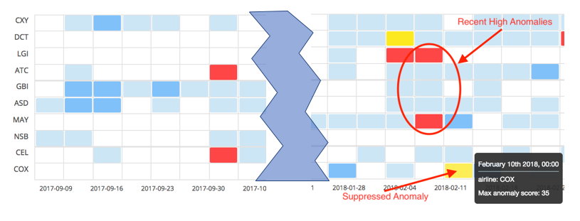
We can see that in the recent past, critical anomalies were detected in two other partitions, airline:LGI and airline:MAY. If we were to drill in and look at those two airline’s anomalies in detail, we would see that they have probability values much smaller than the anomaly for airline:COX. As such, it was deemed that the anomalies for the other airlines were more serious and thus deserved the higher normalized scores. Again, the normalization tables were global across all partitions.
Maximum Normalized Score Per Partition in 6.5
Now, in the 6.5 release, we have made a subtle change that brings significant effects. We now keep track of maximum normalized score scoped to each partition. This is not a full normalization table for every partition, which would likely be too much overhead for jobs with lots of partitions. Instead, this new approach gives nearly a similar effect, without the burden of much additional overhead. Let’s see how things have changed.
In version 6.5 the results of the single metric job for airline:COX again still shows a significant anomaly at the point of interest:
The anomaly score of the highlighted point of interest is scored with a 65 - this in itself is different than the score given in version 6.4, but this is due to other changes to the machine learning analytics (including multi-bucket, described later). Let’s compare apples to apples and see what this point in time is scored when the other airline partitions are added in with the multi-metric job:
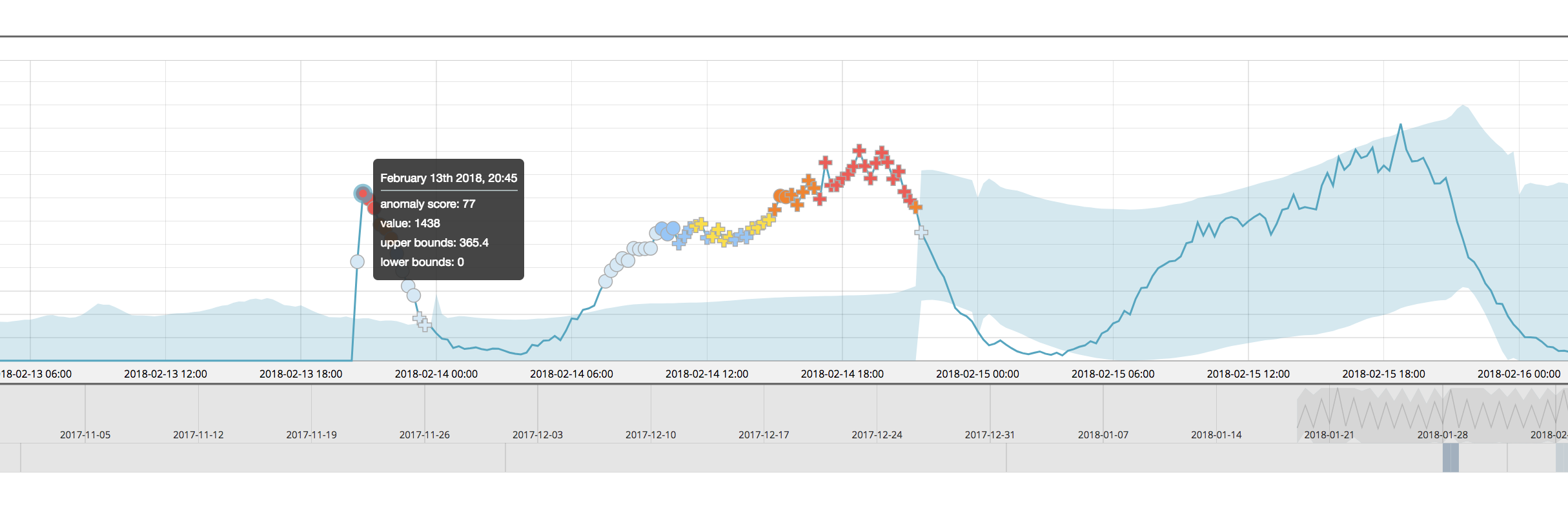
The normalized score for airline:COX is 77, even when the job is partitioned. This is much more similar to the score of that for the single metric job and thus demonstrates that the partitions are normalized more independently than in versions prior to 6.5.
The overall effect of the change to normalization in 6.5 is to produce a much wider range of scores. This can, again, be best seen by looking at the Anomaly Explorer view:
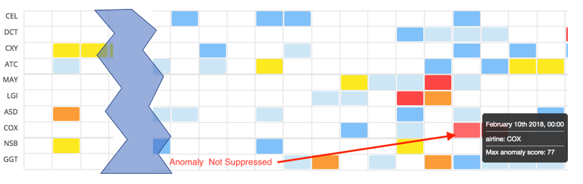
There is now a greater number of minor and major anomalies (yellow and orange cells).
Using a range aggregation we can easily determine the distribution of the normalized anomaly scores over the severity types for both 6.4 and 6.5.
GET /.ml-anomalies-shared/_search
{
  "size": 0,
  "query": {
    "bool": {
      "must": [
        {
          "match": {
            "result_type": "record"
          }
        },
        {
          "match": {
            "job_id": "data_high_count_by_airline"
          }
        }
      ]
    }
  },
  "aggs" : {
        "score_ranges" : {
            "range" : {
                "field" : "record_score",
                "ranges" : [
                    { "to" : 25.0 },
                    { "from" : 25.0, "to" : 50.0 },
                    { "from" : 50.0, "to" : 75.0 },
                    { "from" : 75.0 }
                ]
            }
        }
    }
}
The results are summarized in the table below.
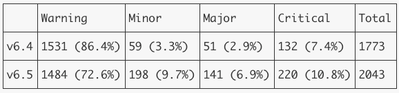
Clearly, in 6.5 there are more anomalies created overall, and scores are shifted higher in the severity scale.
While we don’t always recommend setting alerts that trigger off record scores, we are aware that some Elastic machine learning users do so. It is therefore worth noting that the changes to normalization should make existing record level alerts fire more frequently. It is advised that alerting logic in machine learning-based Watches are reviewed once 6.5 is in place.
Multi-Bucket Analysis
Sometimes interesting events don’t exist solely within a single bucket span — they may instead occur over a range of contiguous buckets — making the short-term trend unusual. In the past, the only way of detecting such cases would be to have the machine learning job with a longer bucket span (or run several jobs on the same data with varied values of bucket span). This was not always practical and improvements were needed.
For example, below we see the single metric view for a job run in 6.4
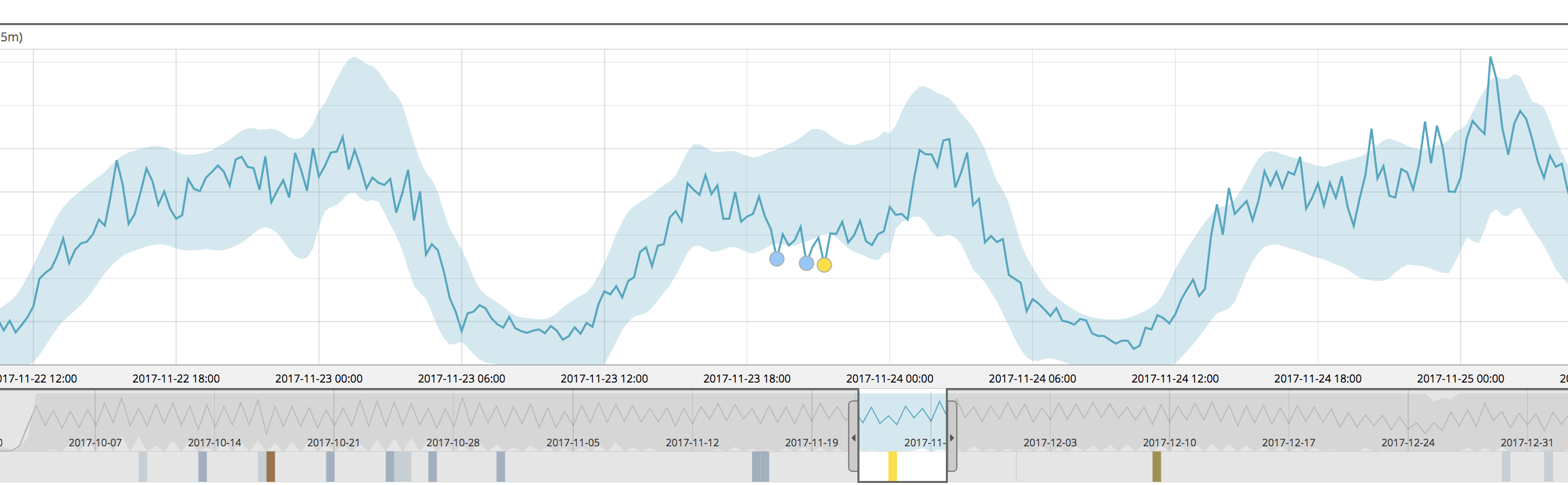
This job was configured to detect lower than expected counts of indexed documents — and we see that it has found a few minor anomalies in the selected time window, but the overall sag in volume mid-day wasn’t really prominently identified.
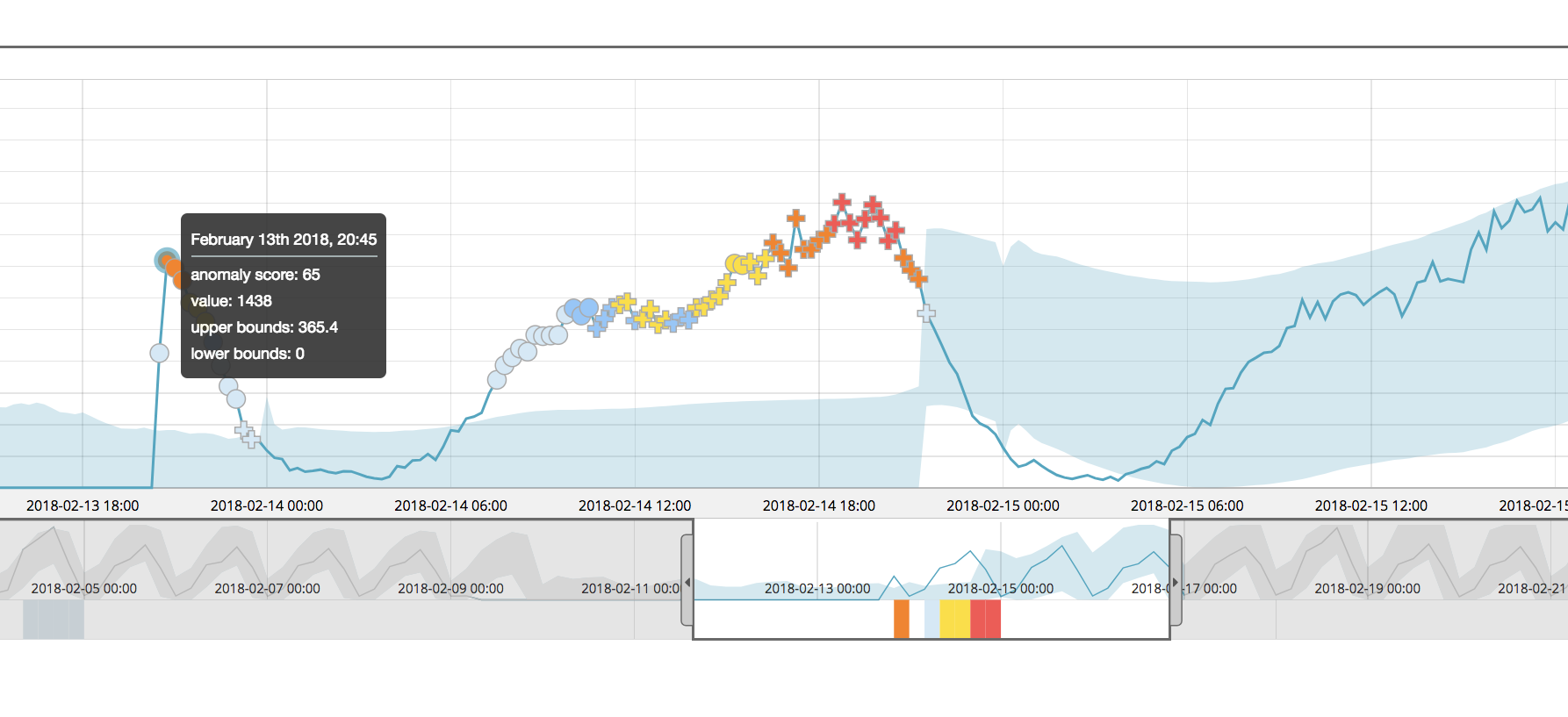
In a version 6.5 multi-bucket analysis, we see that the mid-day sag is now flagged more seriously:
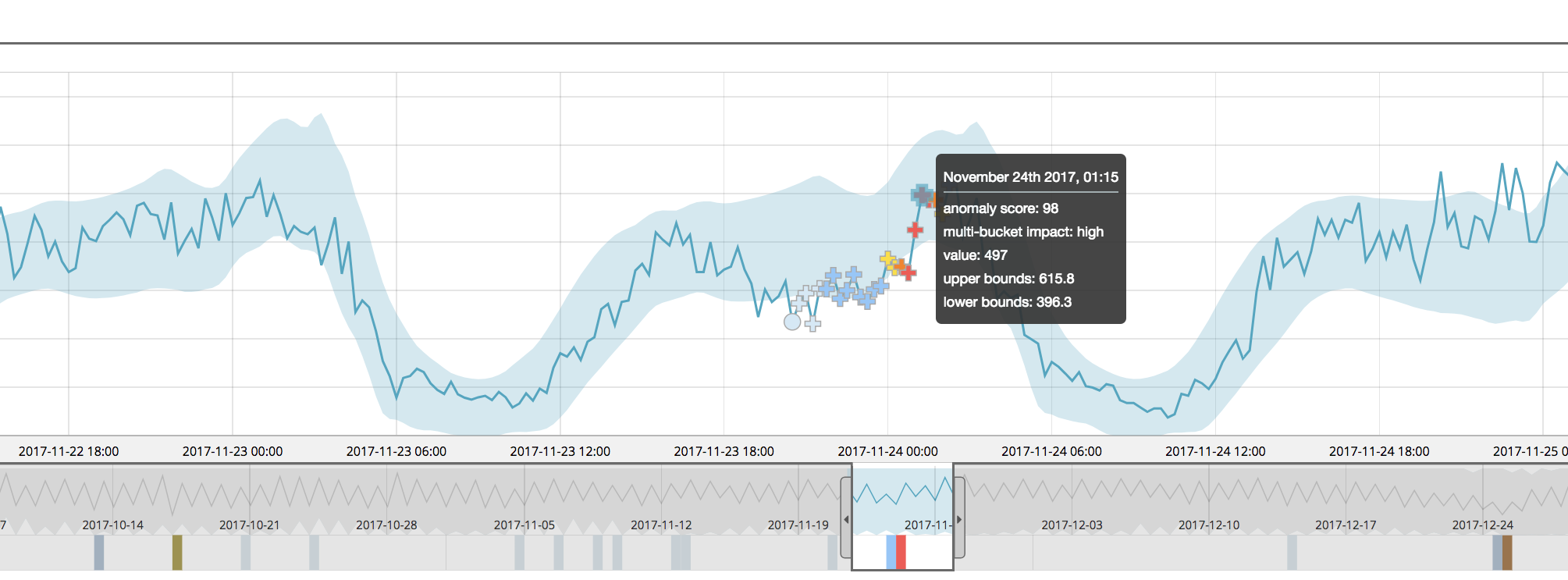
Notice that the multi-bucket anomalies are now indicated by a new “cross” symbol in the UI.
Note: An additional quirk can occur with multi-bucket anomalies — they may sometimes appear to be “inside the bounds” of the model (if the bounds are on). If you see this, this is not an error — it is just that the model bounds are calculated per bucket, so they’re not applicable to a multi-bucket view of the data.
Under the hood, we calculate the impact of multi-bucket analysis on the anomaly and rank it from -5 (no multi-bucket contribution) to +5 (all multi-bucket contribution). There is also now text for high, medium or low multi-bucket impact included in the anomaly marker tooltips as well as in the expanded row section of the anomalies table.
When querying the .ml-anomalies-* indices for record results (for alerting or other non-UI purposes), we now report the value of this new multi_bucket_impact field:
{
  "_index" : ".ml-anomalies-shared",
  "_type" : "doc",
  "_id" : "data_low_count_atc_record_1511486100000_900_0_29791_0",
  "_score" : 8.8717575,
  "_source" : {
    "job_id" : "data_low_count_atc",
    "result_type" : "record",
    "probability" : 5.399816125171105E-5,
    "multi_bucket_impact" : 5.0,
    "record_score" : 98.99735135436666,
    "initial_record_score" : 98.99735135436666,
    "bucket_span" : 900,
    "detector_index" : 0,
    "is_interim" : false,
    "timestamp" : 1511486100000,
    "function" : "low_count",
    "function_description" : "count",
    "typical" : [
      510.82320876196434
    ],
    "actual" : [
      497.0
    ]
  }
}
Wrapping Up
In conclusion, these two changes to scoring will be quite meaningful to users who previously thought that Elastic machine learning “didn’t score anomalies high enough” for certain situations. This change also highlights our seemingly never-ending pursuit of making our anomaly detection best-of-breed.
If you’d like to try machine learning on your data, download the Elastic Stack and enable the 30-day trial license, or start a free trial on Elastic Cloud. And, if you are trialing the software and have questions, feel free to seek help on our public discussion forums at discuss.elastic.co.