Elasticsearch has native integrations with the industry-leading Gen AI tools and providers. Check out our webinars on going Beyond RAG Basics, or building prod-ready apps with the Elastic vector database.
To build the best search solutions for your use case, start a free cloud trial or try Elastic on your local machine now.
Elasticsearch is introducing a new type of vector in 8.6! This vector has 8-bit integer dimensions, where each dimension has a range of [-128, 127]. This is 4x smaller than the current vector with 32-bit float dimensions, which can result in substantial space savings.
You can start indexing these smaller, 8-bit vectors right now by adding the element_type parameter with the byte value to your vector mappings, similar to the example below.
But what if your existing vectors' dimensions don't fit into this smaller type? Then we can use the process of quantization to make them fit, often with only a small loss of precision!
Let's quantize
Let's start by defining quantization. Quantization is the process of taking a larger set of values and mapping them to a smaller set of values. More specifically, in our case this would be taking the range of a 32-bit float and mapping it to the range of an 8-bit integer for each dimension in a vector. (This should not be confused with dimensional reduction, which is a different topic. This is only reducing the range of the values for the existing dimensions.)
This leads to two further questions. What is the actual range of our 32-bit float vectors? And what function should we use to do the mapping? The answers vary significantly based on use-case.
As an example, one of the simplest forms of quantization is taking the dimensions of normalized 32-bit vectors and linearly mapping them to the full range of the dimensions of 8-bit vectors. Using Python, this would look something like the following:
This is only a single example, though. There are many other useful quantization functions. For your specific use case, it's important to evaluate what method of quantization will give you the best results relative to the trade-off between space reduction, relevance, and recall.
Some real-world numbers
8-bit vectors and quantization are great and all, but do they really reduce space in a real-world use case? The answer is unequivocally YES! And substantially. This is all while they continue to give good results without hurting relevance and recall. Elasticsearch even has all the tools you need to do that evaluation yourself with our rank evaluation API.
Now, let's look at some numbers generated from a real-world example with the following setup:
- All data was gathered using Elasticsearch in Cloud with two gcp.data.highcpu.1 64GB nodes
- Data was collected from the NQ dataset (Natural Question), built by Google, used in BEIR
- The embeddings model was sentence-transformers%2Fall-MiniLM-L6-v2
- Quantization to generate 8-bit integer vectors was applied to the 32-bit float vectors collected from the data using the previous example Python snippet
Then we make some magic happen and collect results based on this setup:
| category | Median kNN Response Time | Median Exact Response Time | Recall@100 | NDCG@10 | Total Index Size (1p, 1r) |
| byte | 32ms | 1072ms | 0.79 | 0.38 | 5.8gb |
| float | 36ms | 1530ms | 0.79 | 0.38 | 16.4gb |
| % Reduction | 11% | 30% | 0% | 0% | 64% |
And our results look fantastic. Let's break down each one.
- Median kNN Response Time: This response time is collected using approximate kNN search against our example data set. This type of search uses Lucene's HNSW graph as the backing data structure. We see an 11% increase in response time for byte versus float.
- Median Exact Response Time: This response time is collected using exact kNN search against our example data set. This type of search uses a script to iterate through every vector in the data set and will return the best possible results. We see a large improvement of 30% reduction in response time!
- Recall@100: This shows us if the most relevant results are included in the top 100. This is important to show if our quantization function worked well. We can see that the numbers are identical for byte versus float, which means that our relevance even after quantizing is just as good for byte as it is for float.
- @NDCG@10: This shows us how good the quality of our first 10 results is. This is another important metric to evaluate if our quantization function worked well. Once again, the numbers are identical between byte versus float, so we can rest assured that our results are still just as good even after quantization.
- Total Index Size (1p, 1r): This is the total index size used for our vectors' index with a single partition and a single replica. For this metric, we disabled source, which we recommend for all vector fields in which the ingested vector data is unmodified so it's not stored twice. And we see a massive 64% reduction in total index size! This doesn't quite reach the 4x difference between a byte and float because of additional overhead for the HNSW data structure including graph connections, but it's still a quite substantial size reduction.
Byte vectors are all ready to go as part of 8.6, and we encourage you to fire up a cluster in Elastic Cloud and give them a try!
Related Content

Describe it, don't draw it: AI-native Kibana dashboards via MCP and ES|QL
From prompt to dashboard. Learn how to build Kibana dashboards with natural language, using example-mcp-dashbuilder: an open source MCP application that writes ES|QL queries, creates interactive charts and exports fully functional dashboards directly to Kibana.

March 13, 2026
Entity resolution with Elasticsearch, part 4: The ultimate challenge
Solving and evaluating entity resolution challenges in a highly diverse “ultimate challenge” dataset designed to prevent shortcuts.

March 4, 2026
Entity resolution with Elasticsearch, part 3: Optimizing LLM integration with function calling
Learn how function calling enhances LLM integration, enabling a reliable and cost-efficient entity resolution pipeline in Elasticsearch.

February 26, 2026
Entity resolution with Elasticsearch & LLMs, Part 2: Matching entities with LLM judgment and semantic search
Using semantic search and transparent LLM judgment for entity resolution in Elasticsearch.
February 18, 2026
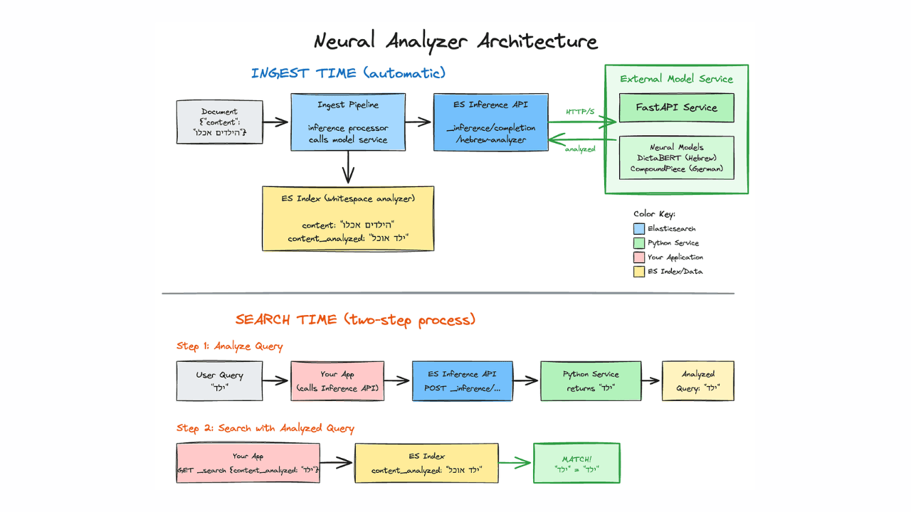
Better text analysis for complex languages with Elasticsearch and neural models
Using neural models and the Elasticsearch inference API to improve search in Hebrew, German, Arabic, and other morphologically complex languages.