How to analyze and optimize the storage footprint of your Elastic deployment

Have you ever looked at your indices and wanted more detail on what is driving storage consumption in your Elastic deployment? Perhaps you have ingested custom data using default settings and would like to know where your data modeling efforts could make the largest impact? In this blog post we will look at how to use Elastic’s recently introduced disk usage API to answer such questions.

Here at Elastic, when we work with our customers, one of the most common areas of improvement is index mapping configuration. A lack of mappings, or using the wrong types, can increase storage usage in your Elastic deployment. This post will help you understand what fields are most influential in driving your storage footprint and how you can optimize consumption through best-practice configuration.

Getting started

If you are not already using Elastic, create a deployment using our hosted Elasticsearch Service on Elastic Cloud. The deployment includes an Elasticsearch cluster for storing and searching your data, and a Kibana instance for visualizing and managing your data. For more information, see spin up the Elastic Stack. I recommend using a development or staging environment for this exercise.

You will also need some data in an Elasticsearch index to analyze. If you have created a brand new cluster, you can add some sample data using Kibana. In my example, I have used some log data ingested using Filebeat.

If you are using Elastic’s Beats or Elastic Agent to index data, chances are it will already be modeled according to Elastic’s best practices. This is of course fantastic, except it does make this exercise a bit less interesting. Fortunately we can easily discard our data model by copying it to an index without a mapping configuration. I picked one of my indices and executed the following reindex operation using Kibana dev tools:

POST _reindex/
{
  "source": {
    "index": "filebeat-7.16.2-2022.01.06-000001"
  }, 
  "dest": {
    "index": "nomapping-filebeat"
  }
}

Note that I have chosen a target index name that starts with a prefix that does not match any of Elastic’s standard index patterns. This ensures mappings are not automatically applied from one of my index templates.

By having two copies of the index, one with appropriate mappings and one without, we will be able to do a side by side comparison later in the blog post.

The final prerequisite is jq, which is a great tool for manipulating json. We will use jq to transform the API response into a list of documents, which we can easily ingest into Elasticsearch using Kibana. This will make the analysis of the API response easier using the Discover interface through Kibana.

Using the disk usage API

Calling the disk usage API is simple, just go to Kibana dev tools and issue a request similar to:

POST nomapping-filebeat/_disk_usage?run_expensive_tasks=true

Note the run_expensive_tasks parameter is required ,and by providing it I acknowledge that I am putting additional load on the cluster. This is also the reason for my earlier recommendation to do the exercise in a non-production cluster.

Here is the top of my response:

{
  "_shards" : {
    "total" : 1,
    "successful" : 1,
    "failed" : 0
  },
  "nomapping-filebeat" : {
    "store_size" : "23.3mb",
    "store_size_in_bytes" : 24498333,
    "all_fields" : {
      "total" : "22.7mb",
      "total_in_bytes" : 23820161,
      "inverted_index" : {
        "total" : "9.9mb",
        "total_in_bytes" : 10413531
      },
      "stored_fields" : "8mb",
      "stored_fields_in_bytes" : 8404459,
      "doc_values" : "3.1mb",
      "doc_values_in_bytes" : 3284983,
      "points" : "1.1mb",
      "points_in_bytes" : 1237784,
      "norms" : "468.1kb",
      "norms_in_bytes" : 479404,
      "term_vectors" : "0b",
      "term_vectors_in_bytes" : 0
    }

The response provides a breakdown of the storage usage of the index as a whole. We can see that the inverted index is the largest factor, followed by stored fields and doc values.

Looking further down the response, I get a breakdown of each field, including the host.name field.

"fields" : {
…
"host.name" : {
        "total" : "23.2kb",
        "total_in_bytes" : 23842,
        "inverted_index" : {
          "total" : "23.2kb",
          "total_in_bytes" : 23842
        },
…

We could easily be satisfied with the API results. By using the CTRL-F function in the response tab and searching for “mb”, as in megabyte, we would quickly identify a few large fields in our index. Let’s take it one step further though and look at how we can quickly reformat the response and analyze it using Kibana.

Analyzing field disk usage in Kibana

Copy paste the API result into your favorite text editor and save it as a file, in my case disk-usage-filebeat.json. Then run the command below, replacing nomapping-filebeat with your index name and disk-usage-filebeat.json with your recently saved file:

jq -c '.["nomapping-filebeat"].fields | to_entries | map({field: .key} + .value) | .[]' disk-usage-filebeat.json > disk-usage-ld.json

The command transforms the json into a list of objects, each including a field name and related usage data, and outputs newline delimited json. See the jq manual for more information.

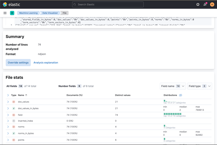
We can now upload the data using the data visualizer, found under **Machine learning **in Kibana. Once you have navigated to the visualizer, click import file and upload your disk-usage-ld.json file. The resulting page should include fields similar to the screenshot below, matching the field analytics in the API response.

Scroll down, click import and name your index where the disk usage data will be stored. Make sure to check the “create index pattern” tick box.

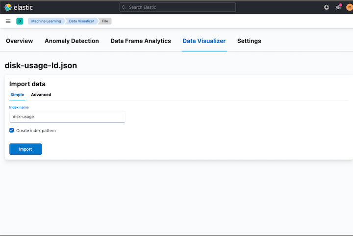
As you can see I named my index disk-usage. On the next screen click** Index Pattern Management**. You can also navigate using the main menu: Stack Management -> Index Patterns.

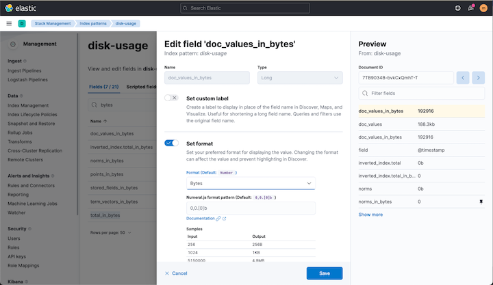
We will use the formatting feature in Kibana to improve the readability of our byte fields. For each of the following fields click edit and select bytes as format:

• doc_values_in_bytes
• inverted_index.total_in_bytes
• stored_fields_in_bytes`
• total_in_bytes

Tip: enter bytes in the search field to quickly find the fields, as in the following screenshot.

Now we are ready to visualize our field data. Navigate to **Discover **and select the **disk-usage **index pattern. Add the following columns:

• field
• stored_fields_in_bytes
• inverted_index.total_in_bytes
• doc_values_in_bytes
• total_in_bytes

Sort on **total_in_bytes **in descending order.

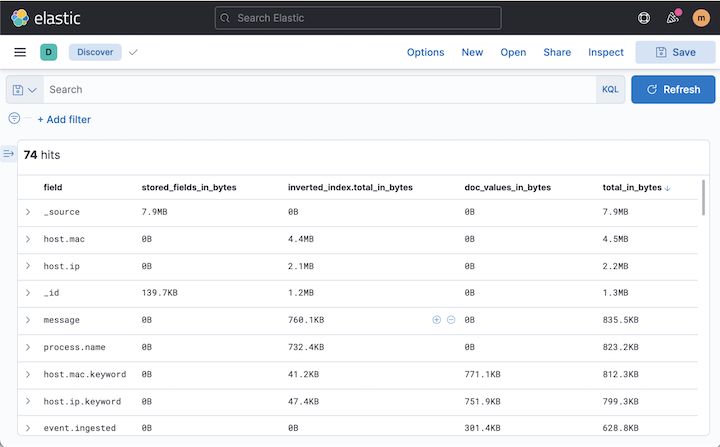
As you can see my largest field is **_source. **This is a built in field that stores the original document, and one we almost always want to keep. The next two fields are **host.mac **and **host.ip. Looking further down we can also see **the same fields with a **.keyword **suffix. As per Elasticsearch's dynamic mapping defaults, these fields have been set to text with a keyword multi-field. I also notice that the text fields’ storage is taken up by the inverted index, which is used for search, while the keyword fields’ are dominated by doc_values, which are used for aggregations and sorting.

Adding the text and keyword sizes together, the total sizes are:

• host.mac + host.mac.keyword = 5.3 MB
• host.ip + host.ip.keyword = 3 MB

Comparing to Best Practice

Lets navigate to **Dev tools and take a **look at the original filebeat index. This index has the Elastic Common Schema mapping already applied out of the box.

I retrieve the disk usage information from my original index using:

POST filebeat-7.16.2-2022.01.06-000001/_disk_usage?run_expensive_tasks=true

From the response I read the following for the **host.ip **and host.mac fields:

"host.ip" : {
        "total" : "1.3mb"
…
"host.mac" : {
        "total" : "492.1kb",
…

As we can see, the storage usage is lower by a factor of 2-5. To take a look at the mapping, we can retrieve it using:

GET filebeat-7.16.2-2022.01.06-000001/_mapping/field/host.ip,host.mac

I can see that host.ip is mapped as ip and host.mac is mapped as keyword. In most cases, the type of data stored in these fields will be used for exact filtering, aggregations and sorting which means that having them mapped as a text field does not provide further value for analysis and takes up extra storage space in the cluster.

Conclusion and Next Steps

In this blog post we have seen how we can use the disk usage API to understand what fields are most expensive in terms of storage utilization. We formatted the API response using jq and imported it back into Elastic using the data visualizer so that we could analyze the data in Discover. We have also seen how having an appropriate mapping can dramatically reduce the storage footprint. So how do we optimize storage usage in our indexes?

Use Elastic Integrations

By using Elastic integrations, either through Beats or Elastic Agent, field mappings will be automatically created for you as data is ingested. Please note that if you don’t send data to Elasticsearch directly, for example if you send Filebeat data via Logstash, you might need to load your index templates manually.

Configure Mappings

If you are using custom data, you often need to configure your mappings manually. To make sure your mapping is applied, define it within an index template with the appropriate index patterns.

Mapping individual fields quickly becomes tedious. For most machine generated data we usually want to map most strings to the keyword type, so including a dynamic template as the example below will save a lot of time. Don’t forget to add specific mappings for ips and for text meant for free text search, such as the standard field “message”.

"mappings": {
    "dynamic_templates": [
      {
         "strings_as_keyword" : {
           "match_mapping_type" : "string",
           "mapping" : {
             "ignore_above" : 1024,
             "type" : "keyword"
           }
         }
       }
    ]
  }

When naming and assigning types to your fields we recommend consulting the Elastic Common Schema. It will help you build a consistent data model and allow you to view your custom data in Kibana’s applications.

Implement Storage Tiers

A slightly tangential, but important, tool to optimize your storage footprint is data tiers. By using data tiers you can move data to cheaper hardware as it ages. Our frozen tier even lets you store data in blob storage, which dramatically reduces costs and is designed for data that is rarely accessed or when slower query responses are acceptable. The easiest way to manage data tiers is by using Elastic Cloud, have a look at our best practices for managing data to get you started.