Benchmarking outlier detection results in Elastic machine learning
Outlier detection aims to identify patterns in data that separate normal from abnormal data points. It has extensive applications for intrusion detection and malware identification in security analytics, fraud detection, and customer behavior analysis. In these cases, time is not necessarily an important component in your analysis. For example, a credit card user based in New York City might have gotten a holiday bonus, and as a result, increased their average spending with respect to time but otherwise is behaving normally. This increase in spending may be abnormal, but they’re still spending at the same stores in the same neighborhoods. If we then see a transaction that comes from a gas station in California (our New Yorker doesn’t own a car), we might suspect that something is up.
Outlier detection utilizes the recently released Transforms capability. With transforms, you can create an entity-centric view of your data — allowing you to perform feature engineering with Elasticsearch aggregations. Continuing with the credit card example, if our data comes in as individual transactions, we can pivot our data around a customer_id field, and create features that uniquely define a customer, like their total spend, their monthly spend, the number of distinct merchants they shop at, and the number of geo_locations in which they have activity. Passing this transformed data to outlier detection would allow the credit card company to identify accounts that are potentially compromised.
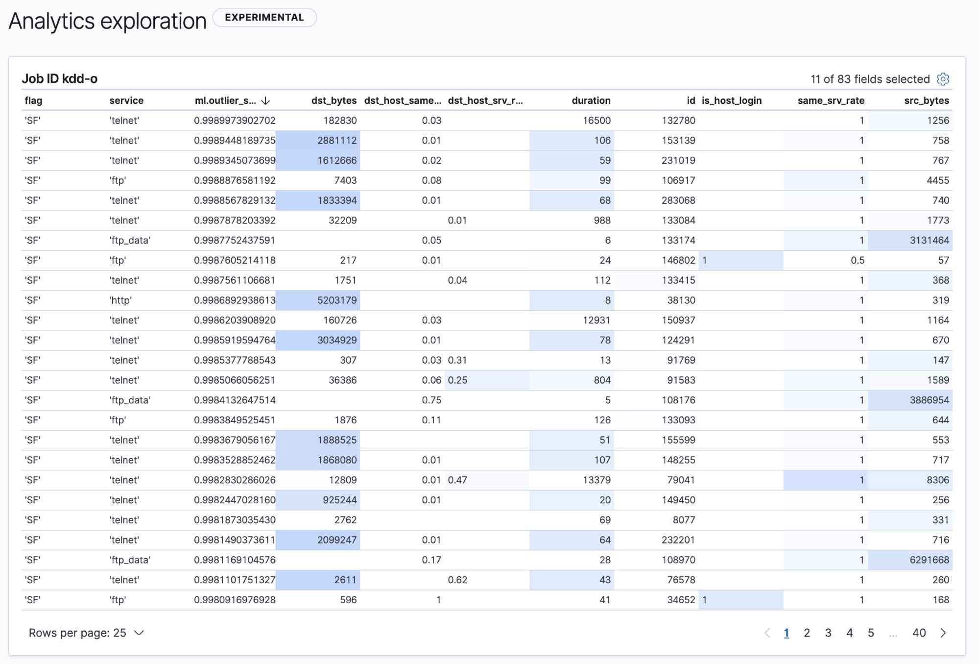
An API for outlier detection was released as experimental in 7.3, and with 7.4, we’ve released a dedicated UI in machine learning for performing outlier detection.
Outlier detection, the Elastic way
You might wonder how this differs from our population jobs. The main difference here is that outlier detection can run on data that isn’t a time series, and it can work with an arbitrary number of features. Population detection is an anomaly detection job that analyzes a single feature and requires there to be a time dimension in the data. With population analysis, we often suggest that populations be as homogenous as possible; there is no such requirement with outlier detection.
So how do we do it? Our outlier detection offering is based on an ensemble of learners. There are several quantities that go into creating our ensemble:
- Method — Currently we have a collection of nearest neighbor methods: some based on local density (LOF, LDOF), and some based on global density (kNN, tNN).
- Hyperparameters — Currently we have the number of neighbors in the neighborhood as a hyperparameter.
- Down sample — We can choose a random subset of points for which to compute neighborhoods. This has proven to be effective in empirical studies, as it allows each individual learner to see a different portion of the dataset, which reduces the effects of masking.
- Project — We want some form of dimension reduction to deal with many features; our current approach is to project onto a random subspace. This is similar to feature bagging, but instead weights the contribution from each feature by a sample from a random variable.
Each of these individual learners predicts an outlier score for the data point, and the final score is a product of the individual outlier scores.
Common outlier detection algorithms
Now that we’ve seen how we approach outlier detection, let’s review the details of distance- and density-based outlier detection methods.
There are several ways to detect outliers in large datasets — our out-of-the-box solution uses an ensemble of methods to achieve high performance without requiring the user to set any parameters. While outlier detection methods differ in implementation, their goal remains the same: when treating each data point as a point in n-dimensional space, find those points which are most different from the others and label them outliers. Algorithms differ in how they define and calculate the concept of most different. Before we compare results, let’s first discuss two methods for detecting outliers in large datasets: distance and density methods. For visual convenience, we'll confine our datasets to two dimensions, but the same principles apply to higher dimensions.
Distance-based detection
Distance based methods judge the outlyingness of a point based on its distance to its neighbors. This relies on the basic assumptions that “normal” data have a dense neighborhood and that outliers are far apart from their neighbors. Let’s look at the K-nearest neighbor (KNN) algorithm, which computes an intuitive measure of outlyingness.
Our dataset is made up of points in two-dimensional space with a few obvious clusters. Intuitively, one would assume that points with a large distance from these clusters should be outliers, and the farther away they are, the greater their outlier score. KNN takes a single parameter k and assigns a score to each point equal to the distance from its kth neighbor.
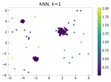
In the figure below, we’ve set k=1, meaning that each point's outlier score is simply its distance to its closest neighbor. We see that there are several relatively isolated points in the lower right that have high outlier scores, which intuitively makes sense. However, we also see a pair of points in the upper right that look like global outliers, but have low outlier scores because they’re right next to one another.
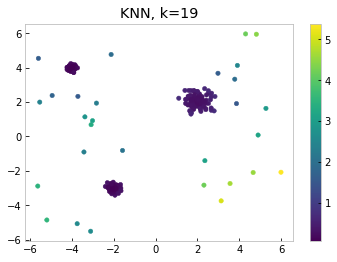
Setting k=19 tells a different story, one that agrees more with our intuition. As one might expect, the lower right points which we identified as outliers in the k=1 case have retained high outlier scores. The pair of points in the upper right corner, whose close proximity to each other caused them to be misidentified as inliers when we set k=1, now also have high outlier scores, which more accurately captures their location in relation to the rest of the data points.
Another thing to note is the KNN does not take into account the density of clusters. In our example, the upper left cluster is much more dense than others. The points around the upper left cluster score relatively low for both k=1 and k=19, even though they are sitting outside the dense region. Therefore, in the region around the dense cluster, these points should be considered to be outlying, even though their distance to the cluster is small globally.
Density-based detection
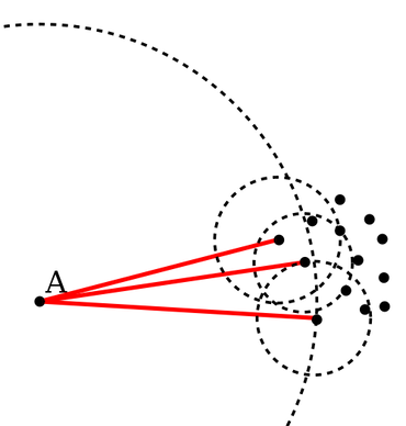
Density-based outlier detection algorithms aim to compare the density around a point with the density around its neighbors. One example of a density based outlier detection algorithm is local outlier factor, which compares the density of a point with the densities of its closest neighbors. In the following figure, the density of point A is a function of its distance to its three nearest neighbors. The densities of these three points are also calculated, and the results compared. Since A’s neighborhood is quite vast (indicated by the larger dashed circle) compared to its neighbors, A would be considered an outlier.
Let’s look at how local outlier factor scores outliers on the sample dataset from above, setting k=19.
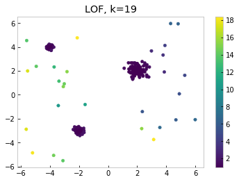

Notice the differences between KNN and LOF in this example. The points in the upper right score low in LOF, since their closest neighbors sit in the least dense cluster. Points sitting outside the upper left cluster, the densest one, score high. Thus we can see that using LOF allows us to capture another important aspect of our dataset, namely the density of the data points.
There is no right answer when it comes to choosing an outlier detection algorithm. Elastic’s outlier detection was developed with the following principles in mind:
- Automatically calibrate hyperparameters (k from above)
- Automatically deal with high dimensional data
- Use of ensemble learning for increased predictive performance
- Extraction of additional insights, including dimensions most likely responsible for a point’s outlier score.
Elastic outlier detection stacks up well against other algorithms
While developing outlier detection, we used a collection of datasets that are commonly used in benchmarking outlier detection algorithms. These datasets cover a number of different use cases: from diagnosing heart disease from medical instrument data, to identifying device malfunctions on space shuttles from sensor data. While the datasets we used are publicly available, the use cases are familiar to our customers.
Each dataset comes in a number of different variants: differing saturation of outliers, different normalization techniques, and the presence or absence of duplicate records. Keeping in line with standard benchmarking practices, the results presented here were performed on variants that have been normalized and deduplicated.
The full datasets can be found here; for the remainder of the blog, the collection of datasets will be referred to as DAMI.
ROC AUC
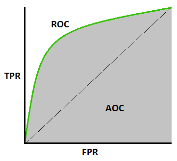
This blog compares each algorithm’s receiver operating characteristic (ROC). For each data point (represented as documents in Elasticsearch), there is a field outlier that is either true or false. The ROC curve plots true positive rates against false positive rates. True positives (or recall) are correctly labeled outliers, and false positives (or fallout) are data points that the algorithm labels as outliers when they are not.
The ROC area under the curve (ROC AUC) is the integral of the curve. A perfect algorithm would have a ROC AUC of 1, and an algorithm that chooses outliers at random would have an ROC AUC close to 0.5.
Comparison of outlier algorithms’ performance
First, we look at Elastic’s out-of-the-box performance against all DAMI algorithms with different choices of k. A total of 1,193 different algorithms were tested to generate the box and whisker plots, covering a variety of different algorithms and parameter values. When running outlier detection with Elastic, no parameters were set — the analysis process automatically sets parameters, requiring no input from the user. This is markedly different from the other algorithms, which require user-supplied values for the parameters. This first plot groups all datasets of the same type, aggregating performance values for different concentrations of outliers (ranging from 2% to 40%) for each dataset.
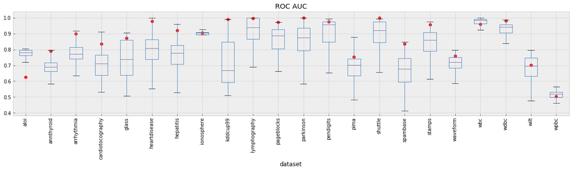
Of the 22 datasets, we see that Elastic’s performance (indicated by a red circle) is in the upper whisker 17 times, within the interquartile range of performance 4 times, and at the low end of performance 1 time. Our suboptimal performance on the ALOI dataset is due to the particular characteristics of the data; ALOI data points form many small, highly dense clusters. Our method of downsampling data when performing outlier detection can lead to false positives. For if we sample only a small number of points from one of the many small clusters, these would be deemed outliers, since most of their closest neighbors have been sampled out. In this way, we've potentially lost an important aspect of what identifies points as unusual.
However, the benefits of downsampling far outweigh the potential drawbacks. For one, downsampling greatly improves the scalability of our algorithm. And in most cases downsampling improves the quality of results because we don't suffer from masking, whereby a small, dense cluster of unusual points mask one another as outliers.
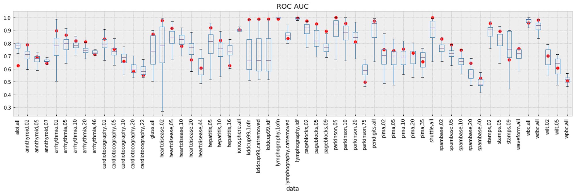
The following figure shows performance across every variant of each dataset. We see that all algorithms tend to perform poorer on datasets with a high concentration of outliers. This is due to the fact that modeling “normal” points in the presence of a high concentration of outliers is more difficult than when there are just a few outlying points.
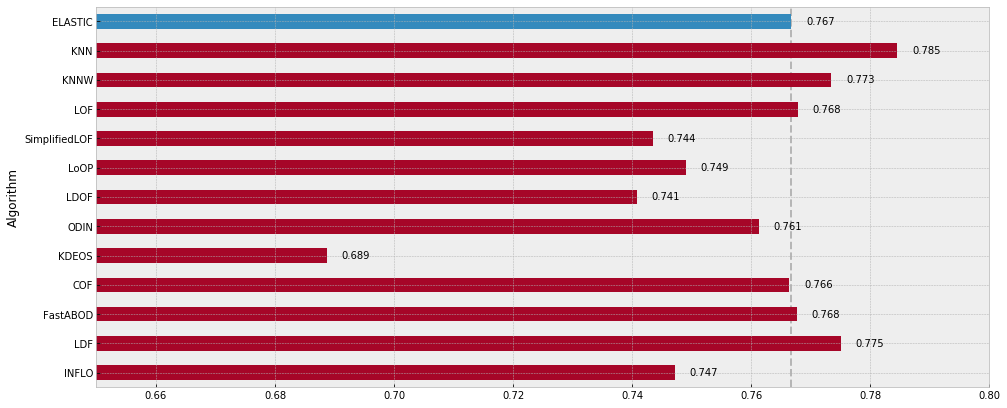
Lastly, we can see each algorithm’s median performance across all of the datasets. Elastic’s algorithm is outperformed by KNN, KNNW, LOF, FastABOD, and LDF when their parameters had been explicitly chosen. However, as no parameters were required to be set for the Elastic algorithm, training was much more seamless.
Conclusion
Outlier detection is our first new analysis type offered since we released anomaly detection. If you'd like to try it out, spin up a free, 14-day Elasticsearch Service trial. We’re really excited to offer a new way for you to find actionable insights from your data, whether or not the data you’re storing is time indexed. We're excited to offer methods that are competitive with state-of-the-art outlier detection algorithms, and would love to hear more about how you are making outlier detection work for your use cases. Enjoy!
For more information about data frames, transforms, and outlier detection, check out this material: