Get hands-on with Elasticsearch: Dive into our sample notebooks in the Elasticsearch Labs repo, start a free cloud trial, or try Elastic on your local machine now.
If you use ES|QL for logs and traces, FROM is probably second nature, but on metrics it can return numerically wrong answers. A query like FROM metrics-* | STATS SUM(request_count) adds up cumulative counter values across every sample on every host. The result grows without bound and isn't a rate, a count, or anything else useful. TS fixes that by grouping samples into time series first, then exposing functions like RATE, AVG_OVER_TIME, and LAST_OVER_TIME that operate per series.
For a high-level tour of metrics analytics across ES|QL and Discover, see Explore and Analyze Metrics with Ease in Elastic Observability. This post zooms in on the mechanics.
Here is the mental model in five bullets:
FROMtreats every document as an independent row. That is right for events, but metric aggregations often need the time series that each row belongs to.TSadds that time series context: it groups and aggregates data points by time series before any other aggregation runs, and enables functions likeRATE,AVG_OVER_TIME, andLAST_OVER_TIME.- A
TS | STATSquery normally has two aggregation phases. The inner phase reduces samples inside each time series; the outer phase groups and combines those per-series results. - The default inner aggregation is
LAST_OVER_TIME, which is whyTS metrics | STATS AVG(cpu_usage)andFROM metrics | STATS AVG(cpu_usage)can return different numbers. - Use
TSto query a time series data stream (TSDS). UseFROMfor events and raw document inspection.
What is a time series, really?
A time series is a sequence of (timestamp, value) data points identified by the metric name and a unique set of dimension values.
For example, request_count reported every 30 seconds by host h1 in data center dc1 is one time series. The same metric on host h2 in dc1 is a different time series.
In a time series data stream, every metric document carries an internal _tsid field that uniquely identifies a time series. Samples that share a _tsid belong to the same time series and are stored sequentially, sorted by timestamp.
That storage layout enables efficient per-series aggregations. It also explains why TS only works on time series data streams. Other index modes have no notion of a time series, so the per-series operations TS relies on have no such identifier to attach to. FROM does not support those operations, which is what the next section is about.
Why FROM leaves metrics on the table
Consider a counter named request_count collected every 30 seconds from three hosts.
A counter is a cumulative metric: each sample is the running total since the process started reporting it. For request_count, a value of 1,000 means "this time series has observed 1,000 requests so far", not "1,000 requests happened since the previous sample". Counters reset to zero on process restart, so a sample of 4 right after 1,004 is a fresh count, not negative traffic. The ES|QL RATE function computes the per-second change within a time series and handles resets without glitches.
You want to calculate the total request rate across all hosts, bucketed by 5 minutes.
If you are used to writing ES|QL over event data, you might start with this query:
The chart it produces looks plausible at first: a line that goes up over time. But the number on the y-axis is the sum of every cumulative counter value reported in the bucket. Each host contributes its own running total, repeatedly, once per sample. Because the query uses SUM on those cumulative values, the result is not a rate, it is not the number of requests in the bucket, and it grows without bound even if the application stops receiving requests.
request_count is a monotonically increasing counter, so its raw values represent "how many requests have ever happened on this host", not how many happened in the bucket. The right computation is "how much did this counter increase per second on each host, then sum across hosts." FROM cannot express that operation directly. It can group rows by fields, but it has no built-in notion of "the same time series over time" and no way to ask for the change of a counter within each time series. It also cannot use sliding-window time series functions such as RATE(request_count, 5m), which we will come back to below.
TS was introduced for this purpose, providing a succinct syntax to express time series aggregations:
RATE(request_count) runs per time series and produces a per-second rate that handles counter resets correctly. SUM then adds those rates across hosts.
Two aggregation phases: inner and outer
Every TS | STATS query has two distinct aggregation phases.
Let's make that concrete with a query that calculates the request rate per data center:
The diagram below shows how TS evaluates this query. It first reduces samples inside each time series, then groups and combines those per-series values into one result per datacenter and time bucket.
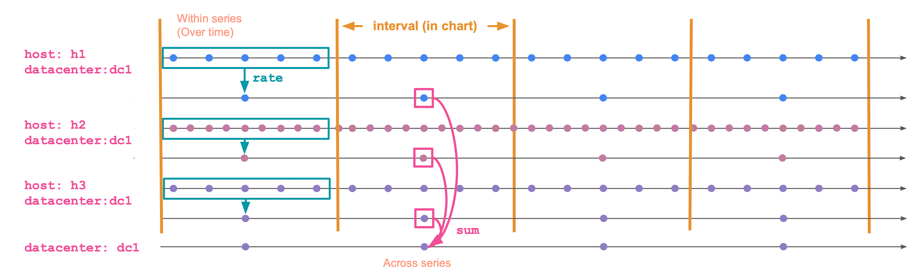
The phases are:
Inner (within a time series). Runs separately for each time series. It collapses many (timestamp, value) data points within a bucket into a single value per time series per bucket by applying the inner aggregation function, such as RATE in the example above. Functions: RATE, AVG_OVER_TIME, MAX_OVER_TIME, LAST_OVER_TIME, STDDEV_OVER_TIME, and so on. The full list is on the time series aggregation functions page.
Outer (across time series, the "grouping" phase). Combines the per-series values into a single value per group per bucket. Functions: SUM, AVG, MAX, MIN, percentiles, and the rest of the regular ES|QL aggregates.
In SUM(RATE(request_count)) BY datacenter, TBUCKET(5m):
RATE(request_count)is the inner aggregation. It runs per time series.SUM(...)is the outer aggregation. It combines time series within the samedatacenterand bucket.TBUCKET(5m)defines the bucket boundaries (equivalent toBUCKET(@timestamp, 5m)).
The outer aggregation is optional. If you only need the per-time-series result, use the time series aggregation function directly:
That query keeps the per-series rate for each bucket instead of wrapping it in SUM, AVG, or another aggregate across time series.
The default inner aggregation: LAST_OVER_TIME
TS has to reduce raw samples inside each time series before it can run the outer aggregation. That means every metric field in a TS | STATS aggregation needs an inner aggregation, even when the query does not spell one out.
Consider a metric named cpu_usage. It is a gauge: a metric that captures a value at a point in time and can move up and down freely. A sample of 0.42 means "this host is at 42% CPU at this time". For a gauge, the natural "value in this bucket" is the most recent sample.
That is what ES|QL fills in for you. If you write TS metrics | STATS AVG(cpu_usage) BY host.name, TBUCKET(5m), the implicit inner aggregation is LAST_OVER_TIME(cpu_usage) and the query is equivalent to:
For each time series, LAST_OVER_TIME picks the latest sample in the bucket. Then AVG averages across time series.
It is also why the same-looking query against FROM and TS can return different numbers. FROM averages every individual document. TS averages one value per time series per bucket. If your hosts publish at slightly different rates, those averages diverge. For example, in a five-minute bucket, a host that publishes every second contributes 300 documents while a host that publishes every two minutes contributes only two or three. With FROM | STATS AVG(cpu_usage), the chatty host dominates the average. With TS, each time series is reduced to one bucket value first, so the outer average gives each host one value to contribute.
If you want the average value during the bucket instead of the latest value, make the inner aggregation explicit:
AVG_OVER_TIME averages all CPU utilization samples within each time series. The outer AVG then averages those per-series values across matching hosts. That makes the result sample-weighted within each time series, then equally weighted across time series. Use this when you care about how the value behaved during the bucket, not just where it ended up.
The same rule applies to peaks and troughs. For a peak CPU chart, use MAX(MAX_OVER_TIME(cpu_usage)), not just MAX(cpu_usage). The inner MAX_OVER_TIME finds the peak within each time series; the outer MAX finds the peak across matching time series.
Counters work the other way around. Their sample value is a running total, so the latest sample on its own is rarely meaningful. For a counter, the inner aggregation you almost always want is RATE for a per-second rate, or INCREASE for the total change in the bucket. Falling back on the default LAST_OVER_TIME gives you the most recent cumulative value, which is the trap the FROM query in the previous section walked into.
Pick the inner function deliberately. The outer function is the easy part.
When to use TS, when to use FROM
A practical rule of thumb:
- Use
TSfor metric aggregations against a time series data stream. It is the source command designed for that data, and it applies per-series semantics by default. - Use
FROMfor events: logs, traces, audit records, transactions. Each row is independent. There is no time series context.
FROM still works on TSDS indices and is occasionally useful, for example when you want to inspect raw metric documents without per-series grouping. For dashboards, alerts, and any kind of charting, TS is the right default.
If you first need to discover which metrics or time series exist in the data, use METRICS_INFO or TS_INFO after TS and before STATS. See ES|QL METRICS_INFO and TS_INFO: Catalog your time series data for a deeper walkthrough.
Post-process TS results with ES|QL
The first STATS command is the boundary between time series processing and regular ES|QL processing. Before that first STATS, TS needs to keep the data grouped by _tsid, so commands that change row order or shape are not allowed. After that first STATS, the output is a regular ES|QL table. You can sort it, limit it, join lookup data, enrich it, or compute derived columns.
For example, this query calculates average CPU per host and bucket, finds the maximum bucketed average for each host, and returns the ratio:
Sliding windows for the inner aggregation
Time series aggregation functions accept a second argument: the window size for the inner phase.
This computes the rate over a 5-minute sliding window, but reports a value every minute. It is useful when you want a smoother chart at fine bucket sizes.
The window is the ES|QL counterpart to a PromQL range vector selector: RATE(app.requests, 5m) serves the same purpose as rate(app_requests[5m]).
Gotchas worth knowing
A few things in TS can seem surprising, especially when coming from the events-based FROM mental model. None of these are bugs; most are direct consequences of the per-series model. Here is what to watch for.
COUNT(*) is rejected. Say you want to know how many samples were collected per service in each bucket. The instinct from FROM is COUNT(*), but TS rejects it: there is no plain "row" once data is grouped by time series, so a row count has no defined meaning. Pick what you actually want to count:
- Number of samples per service:
STATS samples = SUM(COUNT_OVER_TIME(cpu_usage)) BY service.name, TBUCKET(5m). The innerCOUNT_OVER_TIMEcounts samples per time series; the outerSUMadds them across the time series in the group. - Number of distinct hosts reporting per service:
STATS hosts = COUNT_DISTINCT(host.name) BY service.name, TBUCKET(5m). This counts unique label values across time series.
You cannot sort, limit, lookup join, or enrich before STATS. TS metrics | SORT @timestamp | STATS ... will fail. The grouping by _tsid must happen first, before anything else can run. Filter with WHERE if you need to narrow the scope. After the first STATS, the output is regular ES|QL and you can pipe it through any command, as shown in the previous section.
Gauge vs counter mapping. Time series functions are sensitive to the metric type set in the field mapping. RATE only works on counters; *_OVER_TIME functions are intended for gauges. If you build TSDS mappings by hand, pay special attention to this part.
This can be a source of friction for Prometheus users. Prometheus metric type metadata is not always available in the data Elasticsearch receives, so the metric type may have to be inferred from naming conventions (_total for counters, and so on). Those heuristics are imperfect, and a misclassified metric is rejected by the function that should accept it. The deeper mechanics, including how Prometheus Remote Write maps metric types into TSDS, are covered in How Prometheus Remote Write Ingestion Works in Elasticsearch.
Explicit converter functions (gauge-to-counter and counter-to-gauge) are on the roadmap to make these cases easier to recover from at query time.
Kibana charts go empty when you zoom in too far. In Kibana, TBUCKET adapts to the date picker, so zooming in shrinks the bucket size. When the bucket size drops below the data's collection interval, every other bucket has no sample, RATE and the rest return null, and the chart silently goes blank. Elastic is evaluating mitigations such as a runtime warning when the bucket size is too small, a configurable minimum bucket size, or automatic widening of the window or bucket size.
Wrap up
For metric queries, start with TS unless you specifically need raw documents. Then choose the inner aggregation based on what the value should mean inside each time series: RATE for counters, LAST_OVER_TIME for current gauge values, and explicit *_OVER_TIME functions for peaks, averages, minimum values, or distributions.
Once the per-series value is right, the outer aggregation is the familiar part: group and reduce those time series into the chart, alert, or table you need.
For the full reference, see the TS command docs and the list of time series aggregation functions.
Frequently Asked Questions
Why does ES|QL FROM return wrong numbers on counter metrics?
FROM treats each metric document as an independent row, so SUM(request_count) adds up cumulative counter values across hosts and time. The result grows without bound and is not a rate or a count of requests. Use TS with RATE to compute a per-second rate inside each time series, then SUM across hosts.
What is the difference between TS and FROM in ES|QL?
TS is the source command for time series data streams (TSDS). It groups samples by time series before aggregating, which enables functions like RATE, AVG_OVER_TIME, and LAST_OVER_TIME. FROM reads documents as independent rows and has no per-series semantics. Use TS for querying time series data streams, FROM for events and raw document inspection.
Why do TS metrics | STATS AVG(cpu_usage) and FROM metrics | STATS AVG(cpu_usage) return different averages?
TS applies an implicit inner aggregation — LAST_OVER_TIME by default — so each time series contributes one value per bucket. FROM averages every individual document, so a host that publishes 300 samples in a bucket dominates a host that publishes two. The TS answer weights each time series equally; the FROM answer weights each document equally.
How do I compute a per-second rate from a counter in ES|QL?
Use TS with the RATE function: TS metrics-* | STATS SUM(RATE(request_count)) BY TBUCKET(5m), host.name. RATE runs per time series, computes the per-second change, and handles counter resets correctly. The outer SUM then combines rates across hosts.
When should I add a timestamp filter to an ES|QL metrics query?
n Kibana apps that run ES|QL with the global date picker, such as Discover and dashboards, you do not need to add this filter yourself. Kibana applies the selected time range automatically. Outside Kibana, or in Kibana Dev Tools, always add an explicit timestamp filter so the query only scans the time range you intend: WHERE @timestamp > NOW() - 1 hour AND @timestamp <= NOW() or the equivalent shorthand: WHERE TRANGE(1h) TRANGE(1h) is the preferred shorthand for recent time windows. It is equivalent to filtering @timestamp to the last hour, ending at NOW().
What are the two aggregation phases of a TS | STATS query?
The inner phase runs per time series and collapses many (timestamp, value) samples into one value per series per bucket using a time series function (RATE, AVG_OVER_TIME, MAX_OVER_TIME, LAST_OVER_TIME, etc.). The outer phase runs across time series and combines those per-series values using a regular ES|QL aggregate (SUM, AVG, MAX, percentiles). Pick the inner function for correctness; the outer function is the familiar part.
Why does my Kibana metrics chart go blank when I zoom in?
TBUCKET adapts to the date picker, so zooming in shrinks the bucket. When the bucket size drops below the data's collection interval, some buckets contain no sample, RATE returns null, and the chart silently goes empty. Widen the time range or set a longer explicit window in the inner aggregation, e.g., RATE(request_count, 5m).
Can I use SORT, LIMIT, or LOOKUP JOIN before STATS in a TS query?
No. TS must keep data grouped by _tsid until the first STATS, so commands that change row order or shape are rejected before that point. Use WHERE to filter, then STATS, and apply SORT, LIMIT, joins, or enrichment on the regular ES|QL table that comes out of STATS.
Related Content
How to build search analytics on Elastic using OpenTelemetry, no extra pipeline required
How to instrument your search application to use modern Open Telemetry standard to drive insights in to your search and users.
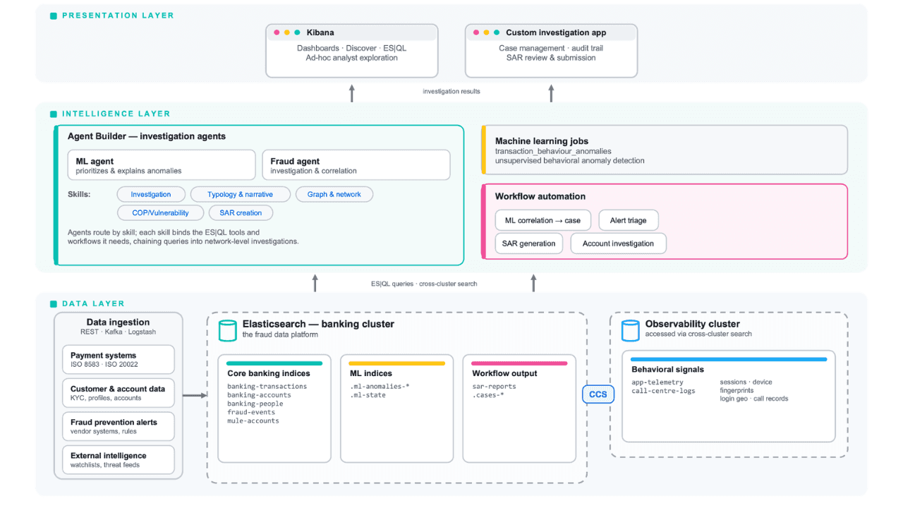
Follow the money: tracing laundering networks with ES|QL and cross-cluster search
The data model, cross-cluster architecture and five ES|QL queries that power mule detection and laundering network tracing, built from infrastructure most financial institutions already run.

July 1, 2026
One command. Natural language. Your Elasticsearch data, straight to the terminal.
Query your Elasticsearch data from the terminal in plain English. The official Elastic GitHub Copilot CLI plugin generates and runs ES|QL queries against your cluster. No Kibana, no manual syntax.
June 30, 2026
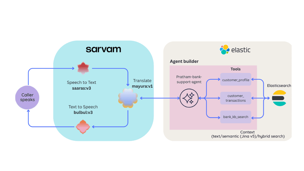
Building a multilingual voice agent with Elastic Agent Builder & Sarvam AI
A working demo combining Sarvam AI speech with Elastic Agent Builder: identity verification, per-customer ES|QL queries, and mid-call language switching across 22 Indian languages without multilingual indices.

June 29, 2026
Bringing it together: How we rebuilt Elasticsearch as a columnar metrics engine; 6.6x less storage, 160x faster queries
Elasticsearch metrics in version 9.4 run on a fully columnar engine: 6.6x less storage, 160x faster queries, native PromQL and OTel support.