Detecting phishing with computer vision: Part 2, SpeedGrapher
Editor’s Note: Elastic joined forces with Endgame in October 2019, and has migrated some of the Endgame blog content to elastic.co. See Elastic Security to learn more about our integrated security solutions.
In the previous post, we discussed the problem of phishing and why computer vision can be a helpful part of the solution. We also introduced Blazar, our computer vision tool to detect spoofed URL. Today we will discuss the second tool we developed that applies computer vision to phishing - SpeedGrapher.

While Blazar focuses on detecting homoglyph attacks (i.e., attacks based on visual character similarity in URLs) with computer vision, SpeedGrapher detects macro-enabled document based phishing. In this post, we describe the growing use of macro-enabled document based phishing and introduce our solution, SpeedGrapher. I presented each of these tools at BSidesLV, demonstrating how Blazar and SpeedGrapher address two often used phishing techniques, while illustrating the power and potential for computer vision to detect phishing.
Overview of Macro-Enabled Document Based Phishing
Phishing attacks can take many forms, one of the most prominent of which exploits the natural tendency to download attachments. In these macro-enabled document based phishing attacks, attackers continue to find success by tricking victims to open malware-embedded documents as attachments in their email. Let’s look at a Word document you could have been emailed.
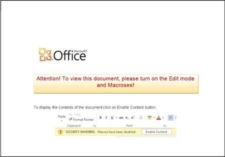
This whole document should throw warning signs. It has instructions on how to “Enable Content” (i.e. enable macros), and includes typos/misspellings such as “Macroses”. These generally are telltale signs of a phishing attack. Enabling content usually sets off a script that downloads a payload to start an attack or sends back valuable information to a C&C server. As we’ve detailed elsewhere, these kinds of attacks with payload delivery have been deployed in some of the most high profile attacks by nation-states, and remain a favorite attack vector by criminals seeking financial gain.
Bounding the Problem Set
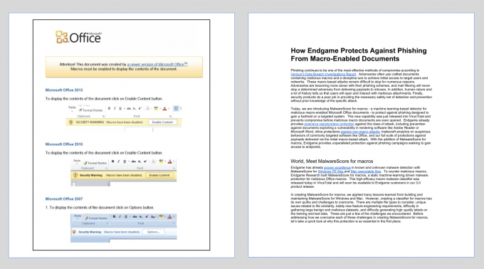
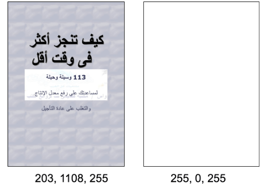
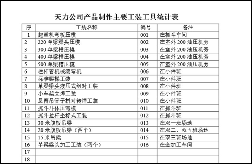
Since this is a vision based exploit, let’s define the problem in a visual way, too. We want to detect the image on the left as malicious and the image on the right as not.

This is the first page of both documents. The one on the left has a lure stating that you can’t read the document due to an incorrect version and requests to “Enable Content”. This is suspicious, especially since the instructions are just an image, and MS Office does not make requests like this. The document on the right is plain text with a few hyperlinks, nothing looking too suspicious except that it talks about macros. Given that many of these suspicious clues are visual, we began creating SpeedGrapher to explore how computer vision may assist in detecting these kinds of phishing attacks.
Getting Started: How We Built SpeedGrapher
As with most computer vision applications, SpeedGrapher is an ensemble of many different techniques. While that sounds complicated, and computer vision in general has an intimidating reputation, this is actually a bonus. Each piece of the solution is relatively straightforward, although some are more complicated than others, and can be understood and completed in chunks. We first need to gather samples and then focus on feature generation.
GATHERING SAMPLES
To get started, the first thing we need to do is gather samples. At Endgame, we have a large sample set from our work in making a macro text based classifier. But you can curate your own set from sources like VirusTotal or other file collection and scanning services.
With the samples in hand, the next step is to capture an image of the first page of the document for clues of malicious activity. One method would be opening the actual file and taking a screenshot of it. However, this is manual and slow. It perhaps could be automated, but that sounds overly complex. Instead, we get a preview from the Word Interop class which contains the logic Word itself uses to interface with a document. Microsoft has great documentation of this here.
Note on safety: With Blazar we were just dealing with strings, now we’re dealing with actual malware. It is worth sandboxing: disable internet, disable macros, enable Windows Exploit Guard for Word.
GENERATING FEATURES
We generated the following features: prominent colors, blur/blank area detection, optical character recognition, and icon detection. Each of these are described below.
Prominent Colors
To calculate prominent colors, we use K-means clustering over the RGB space of the document. We first start with an image:
These images are actually just comprised of a series of pixels with color coding (RGB in our case). We take each pixel and map it into a three dimensional space corresponding to its Red, Green, and Blue values, irrespective of its position in the image. If the image was mostly white, as in this case, we’ll see a lot of data points at the 255, 255, 255 coordinate. If mostly black, we’ll see a lot at 0, 0, 0.
After our data is mapped, we cluster it. K-means clustering is an algorithm that takes the number of clusters, K, as input. We’re going to look for three clusters. The algorithm randomly initializes three clusters in our space and then finds all points that are closer to it than any other cluster center. Next it aggregates those assigned points to find a new centroid, and moves to that position. It then repeats this process (find closest points, aggregate, move, etc) until it reaches steady state or a maximum number of iterations have passed. This produces a set of three color centroids and the corresponding size of their clusters, as you see below
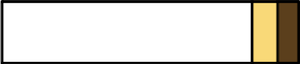
Notice that the largest cluster is white, the next is yellow, and the final cluster is comprised of the little bits of red and black in the image resulting in a brown hue. You can do this yourself by following along with this blog.
Blur Detection
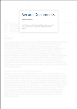
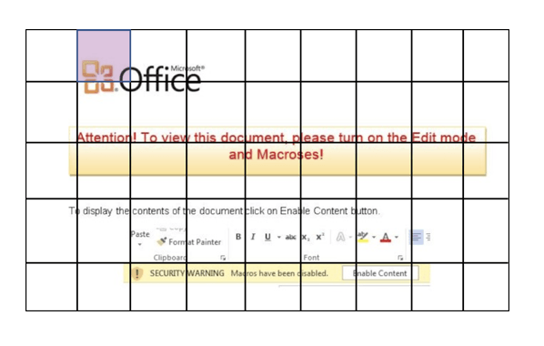
For blur detection we focus on a common technique attackers use to fake the idea that content is hidden. The below document shows a blurred out background with a notification asking the user to “Enable Content” to see the full document. But this is just an image, there is no hidden content.
To measure this, we’re going to find the variation of the Laplacian, which is a second order derivative and measures the sharpness of change. Thinking back to calculus, this is akin to acceleration in the position, velocity, acceleration set. Velocity is the rate of change of position (first order derivative). Acceleration is the rate of change of velocity or the rate of change in change of position (second order derivative).
For a gray-scale image, a white pixel right next to a black pixel right next to a white pixel would have a large measure of sharpness of change. A white pixel with smooth transition of gray pixels to a black pixel would have a small measure of sharpness of change and would also correspond to a blurred image. You can find a guide to do this yourself with this blog.
Blank Detection
Blank detection is a feature that is useful in determining if an attacker is attempting to trick a user with a seemingly broken or corrupt document. We calculate some simple statistics on the average of the RGB values, such as mean, variance, and max. From those values we can numerically show that the image on the left is not blank and the image on the right is blank. Additionally, the mean will tell us what color the blank section is.
Optical Character Recognition
Optical Character Recognition (OCR) is a well worn topic, so we won’t spend time getting into the technical details of translating and converting characters identified in images. There are several technologies that do this well, such as Google’s Tesseract. We decided to use UWP OCR since it was native in Windows 10. Additionally, we implemented text translation via a Google Cloud API to convert as much of the text to English as possible. There are also several other text translation APIs available, like Microsoft’s.
Icon Detection
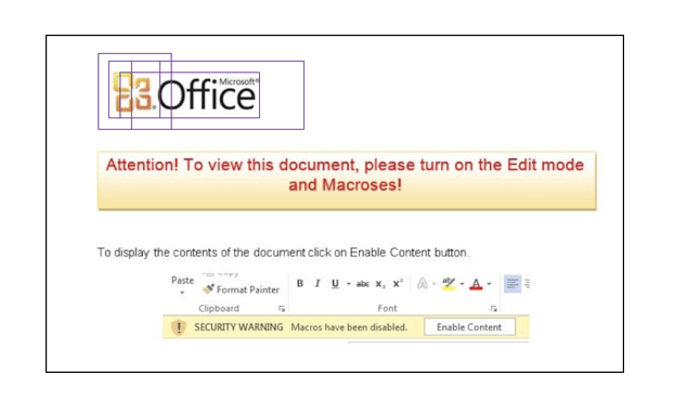
For icon detection, we use YOLOv3. This is a very cool object detection framework. YOLO in this context stands for You Only Look Once, as it scans an image once to determine both image class and bounding box. Please check out the paper and website for more information. We’ll explain it briefly, but they provide much more detail and we highly recommend it.
The general idea is to take an image and section it into cells. Each cell is assigned a probability of fitting with a class from the classes you’re training it to detect. At the same time it is determining possible bounding boxes for objects. It then combines the cell class probabilities and bounding box probabilities to find high confidence predictions and boxes.
For our purpose, we decided to detect five classes of objects that we saw were often used in attacks masquerading as instructions from Microsoft Office:
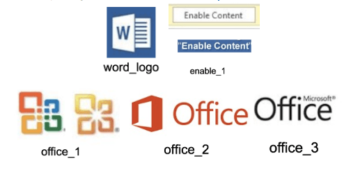
To train, we’ll need 1500 samples with around 300 of each class. We also apply transforms like color shifting and rescaling to make the network robust to these kinds of edits. You can follow along with this blog to train on your own dataset.
If you’re familiar with neural network training, you might immediately realise that 300 samples per class is far too small of a training set for a task of this nature. Generally speaking you would be correct. However, we’re going to leverage Transfer Learning to accelerate our work. Transfer learning in this context is training a network on a large dataset and general task and then adding a final training run on a smaller set with a specific task. The large dataset training time allows the network to learn how to recognize generic features (and importantly be saved and shared), and the small dataset training time focuses the network on the specific task at hand.
For our training we are using this port of YOLO for Windows and a network pre-trained on a large ImageNet set.
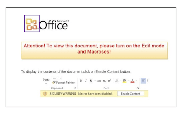
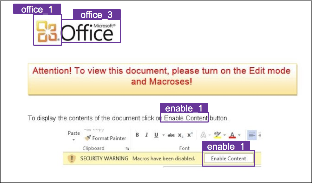
The end result is quite good. We can submit a sample to our YOLO network and get output on any specific icons detected and the confidence in those icon detections. Visually, the identification of icons and determination of their bounding boxes would look like:
COMBINING FEATURES
After all the feature generation is done, we get a json blob for a sample that looks something like:
{
  "sha256": "0a0a5e96f792ab8cae1a79cc169e426543145cb57b74830b548649018a7277f4",
  "data": {
      "img": {"blank": {"data": [253.4725,
                                 118.46424375000001,
                                 255.0],
                        "heur": false},
              "blur": {"data": 470.48171167998635,
                       "heur": false}},
      "top": {"blank": {"data": [243.6475,
                                 1141.22824375,
                                 255.0],
                        "heur": false},
              "blur": {"data": 941.7518285537251,
                       "heur": false}},
      "btm": {"blank": {"data": [254.9825,
                                 0.017193749999999994,
                                 255.0],
                        "heur": true},
              "blur": {"data": -1,
                       "heur": false}}},
  "colors": {"cluster_0": {"centroid": [254.7639097744361,
                                        254.7799498746867,
                                        254.58646616541353],
                           "size": 0.9459503713290462},
             "cluster_1": { "centroid": [178.91304347826087,
                                         127.69565217391305,
                                         116.95652173913044],
                            "size": 0.012234456554165144},
             "cluster_2": {"centroid": [247.4512195121951,
                                        234.0609756097561,
                                        186.8780487804878],
                           "size": 0.041815172116788646}},
  "yolo": ["office_1: 97%",
           "office_3: 88%",
           "enable_1: 87%",
           "enable_1: 95%"],
  "txt": "offit attention! to view this document, please turn on the edit mode and macroses! 0 display the contents of the document click on enable content buttorl p aste format painter clipboard security warning font macros have been disabled. enable content\r\n"
}
Building a Classifier
We’ve put a lot of work into this feature generation, so it only makes sense to build a classifier to make predictions on new samples. To do that we generally need three things:
- Samples - We’ve collected a corpus through various sources
- Feature generator - We’ve documented the creation of several rich feature sets
- Labels - We can use our MalwareScore for Macros labels.
CREATING FEATURE VECTORS
We’re going to take the easy route in this classifier and not conduct a great deal of processing and analysis on our input feature vectors. A lot of that work was done by the feature generation step, and the rest can be done by the classifier algorithm itself. We take the data from our above json blob and smash it all into one 38-dimensional float vector.
color_centroids.sort(key=lambda x: x[1])
color_centroid_vector = []
for cc, s in color_centroids:
    color_centroid_vector.extend(cc)
    color_centroid_vector.append(s)
blank_vector = []
blur_vector = []
for k in ['btm', 'img', 'top']:
    blank_ddata['data'][k]['blank']['data']
    blank_vector.extend()
    blank_vector.append(float(data['data'][k]['blank']['heur']))
    blur = data['data'][k]['blur']['data']
    blur_vector.append(blur)
    blur_vector.append(float(data['data'][k]['blur']['heur']))
yolo_keys = ['enable_1', 'office_1', 'office_2', 'office_3', 'word_logo']
yolo_vector = [0.0, 0.0, 0.0, 0.0, 0.0]
for logo in data['yolo']:
    for yk in yolo_keys:
        if logo.startswith(yk):
            per = float(logo.split(':')[1][1:-1])
            yolo_vector[yolo_keys.index(yk)] = per
text_keys = ['enable content', 'enable macros', 'macros']
text_vector = [0.0] * len(text_keys)
txt = data.get('txt', '')
txt = translator.translate(txt).text
for tk in text_keys:
    if tk in txt:
        text_vector[text_keys.index(tk)] = 1.0
x = np.array(color_centroid_vector + blank_vector + blur_vector + yolo_vector + text_vector)
We use a Random Forest classifier in this example so this step doesn’t matter, but it is good practice to normalize your data to a [0.0, 1.0] scale. This eliminates the correspondence of one feature’s scale to its importance.
import numpy as np
X = np.array(X)
Y = np.array(Y)
high = 1.0
low = 0.0
mins = np.min(X, axis=0)
maxs = np.max(X, axis=0)
rng = maxs - mins
rng = np.array([r if r != 0.0 else 1.0 for r in rng])
X = high - (((high - low) * (maxs - X)) / rng)
Creating, Training, and Evaluating a Classifier
Finally, we create our classifier, train, and evaluate it.
import sklearn.ensemble
n_estimators = 100
max_depth = 6
clf = sklearn.ensemble.RandomForestClassifier(n_estimators=n_estimators, max_depth=max_depth)
for fold in range(nfolds):
    X_train, X_test, y_train, y_test = train_test_split(X, y, test_size=.1)
    clf.fit(X_train, y_train)
    pred_labels_sub = altered_predict(clf, X_test, n_classes)
    pred_vals = [b for (a, b) in clf.predict_proba(X_test)]
    pred_labels.extend(pred_labels_sub)
    y_scores.extend(pred_vals)
    true_labels.extend(y_test)
conf_mat = confusion_matrix(true_labels, pred_labels)
fpr, tpr, thr = roc_curve(true_labels, y_scores)
roc_auc = auc(fpr, tpr)
It is very important to perform cross validation on your dataset as part of the training step to accurately measure your results. We’re using n-fold cross validation, which works by segmenting your data set into n training and evaluation sets. For n=10, we take our entire data set, segment off 10% of it for evaluation, train on the remaining 90%, and then evaluate our hold out set. We repeat this process nine more times, each time picking a different 10% as a hold out. We then aggregate all of our evaluation data to get a very accurate picture of our performance across our entire data set.
plt.plot(fpr, tpr, label='ROC curve of {0} (area = {1:0.2f})'.format('RF', auc))
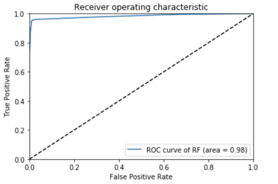
ROC Curve for SpeedGrapher
The AUC of our ROC curve is a respectable 0.98, even without doing anything fancy for our classifier. Further, we examine our confidence matrix to see our True Positives, True Negatives, False Positives, and False Negatives.
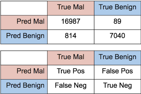
There are 89 false positives in our set, meaning we predict something as malicious when our labels say it is benign. Looking further into these samples we’ve noticed that the majority, around 70%, are actually neutered malware. An example of these neutered samples is below:

It has a macro text of:
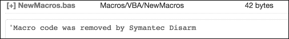
Our detection based on the visual cues was correct, but our ground truth labeling said the sample was benign because the macro text was removed.
Looking at the false negatives, where we call samples benign but are labeled malicious, we find the majority of samples are those that have no visual indication of being malicious. Since our goal here is to detect samples that visually look malicious, these errors largely are expected.
We also don’t handle well samples in some language character sets.
Some are legitimate looking files, like this resume.
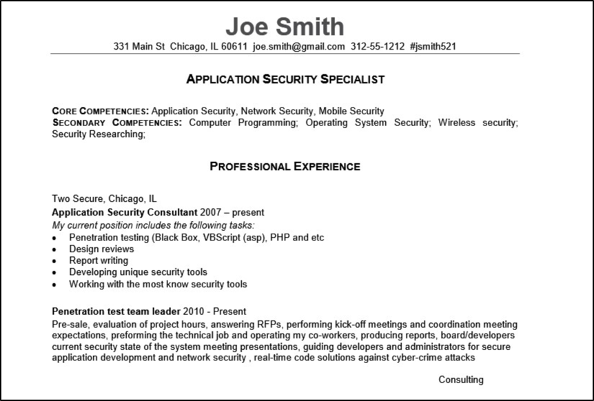
Unfortunately, Joe Smith is doing some nasty work under the hood:
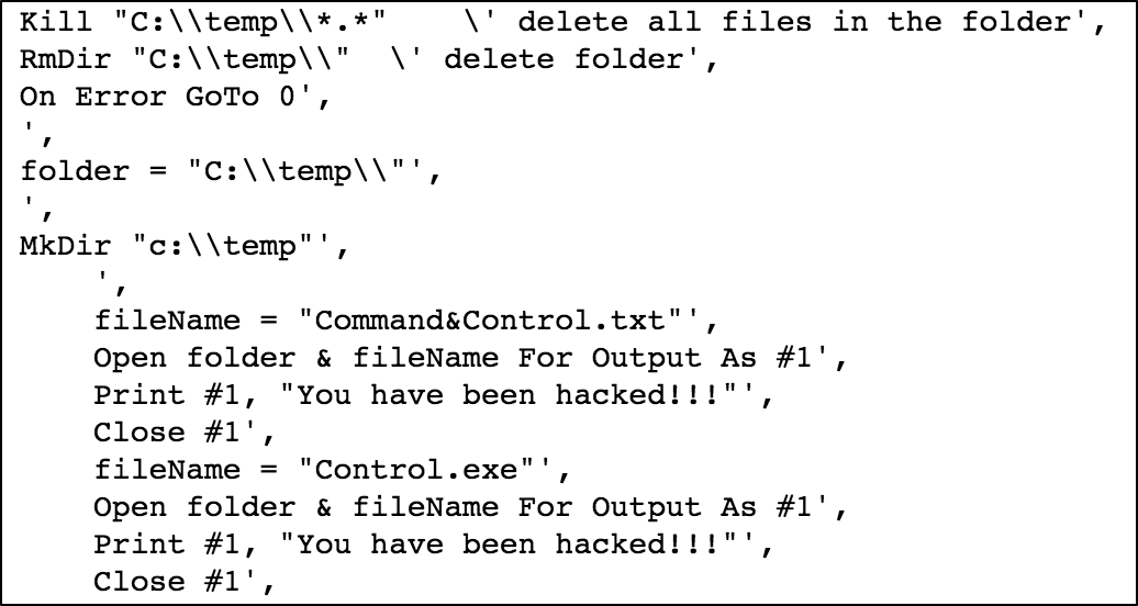
All in all, our classifier, even though not sophisticated, performed quite well due to the rich data we were able to gather from using relatively straightforward computer vision analysis.
Next Steps
In reality, this is our initial model for SpeedGrapher, which we will continue to refine. We’re adding new features, new file types, and lots of secret sauce to continue to improve it. But for the purpose of this blog, we wanted to demonstrate how to easily build a classifier and the benefits of having rich, quality input data.
As the threats evolve and become more complicated to detect, we see computer vision as playing a major role in helping every day users guard against phishing and similar attacks, and we will continue to push the boundary and pursue these innovations.
Happy hunting!