Try out vector search for yourself using this self-paced hands-on learning for Search AI. You can start a free cloud trial or try Elastic on your local machine now.
Elasticsearch's DiskBBQ format (IVF clustering plus binary quantization, built for on-disk ANN search at scale) offers several knobs to shape the recall/cost tradeoff of an index. Automatic calibration seeks to optimize those knobs to achieve optimal performance.
In our previous blog, we laid out the statistical model behind that calibration: a manifold model for how nearest-neighbor distances scale with index size, a Gaussian error model for quantization noise, and a closed-form way to combine the two into an expected recall@k for a given rerank depth. If you haven't read it, the one thing you need going in is this: given a candidate quantization encoding and a rerank depth, we can predict recall@k without building an index and benchmarking it, by fitting two small models to a sample of the corpus.
In this post we’ll go through how to score candidate configurations cheaply and how to leverage that to make merge-time decisions that are themselves cheap, correct, and consistent across real, constantly-merging indexes. This led to some pretty impressive improvements: we see almost 17% average improvement in QPS across a broad range of datasets all while increasing recall (in one case by a factor of 3). What’s more you get this immediately by adding one line to your index options, "auto_calibrate": true, and our plan is to make this our default once it has had the chance to bake a bit.
Why manual vector quantization tuning is unreliable
bbq_disk exposes several knobs: quantization bits for documents (1, 2, 4 or 7), a separate bit width for queries, an oversampling factor for reranking, and whether to precondition vectors before quantizing. None of these act independently, and their effect on recall depends on the data: a 4-bit/1-bit encoding might be plenty for one embedding model and clearly insufficient for another. A single index is also built out of many segments, merged over time, each with an eventually different vector distribution. Hand-tuning one configuration for an entire index is, at best, a compromise, which is the motivation for automatic calibration: let each segment have its own configuration, re-evaluated every time it is involved in a merge operation.
How Elasticsearch runs auto calibration at merge time
When a number of segments are merged and automatic calibration is enabled, Elasticsearch samples documents and queries from the vectors being merged and:
- fits the manifold model over a sequence of nested samples of the merged corpus;
- fits the error model, predicting the quantization error's standard deviation for each candidate
(query bits, document bits, precondition)combination; - sweeps candidate configurations in ascending cost order; the candidate encodings are
(1,1),(4,1),(4,2),(4,4)and(7,7)(query bits, document bits), each tried across oversampling factors of1.25,1.5,1.75,2.0,2.5and3.0; - estimates recall@10 for each candidate using the model described in our first post, and stops at the first (cheapest) configuration predicted to hit the target of 90% recall@10.
The winning configuration (encoding, oversample factor, precondition flag) is stored directly in the segment's metadata, so it travels with the segment and is picked up automatically at query time unless a request explicitly overrides it.
Small segments skip this altogether: below 10,000 merged vectors, there isn't enough data to fit a reliable model, so Elasticsearch just uses the current DiskBBQ defaults (4-bit query / 1-bit document encoding, no preconditioning, 3x oversampling).
How the vector quantization cost model works
Following the principles described in our first post, we started by picking candidates with three nested loops that are essentially how you might imagine hand jamming a lookup table. Start with the quantization scheme as the outer loop, ordered cheapest to most expensive by document bits ((1,1) → (4,1) → (4,2) → (4,4) → (7,7)). Then we set the rerank depth within the middle loop, ordered shallow to deep (1.25× → 3.0×). Finally we set preconditioning within the inner loop (off → on).
That ordering has a cost model baked into it, it's just implicit rather than written down: exhaust every rerank depth at the current bit tier before ever trying more bits. Document bits were effectively the only resource priced as expensive; oversampling was treated as nearly free by comparison, since the sweep would always max out rerank depth on a cheap encoding before considering a pricier one.
The current implementation replaces that with an explicit, continuous cost function:
Query bits still don't factor into cost at all, only document bits (which drive index size) and rerank depth (which drives how many candidates get rescored per query). Preconditioning also stays outside the formula: Elasticsearch runs the whole cost-ordered sweep once with preconditioning off, and only if nothing meets the recall target does it re-run the sweep with preconditioning on, treating it as a fallback lever rather than something priced bit-for-bit against the other two.
With this cost model, rerank depth costs noticeably more per unit than a document bit, so the sweep will often prefer stepping up a bit tier over pushing oversampling deeper.
The main reason for this is that once you're running in a serverless deployment, compute and storage are billed and scaled independently, on very different clocks. An extra document bit is mostly a one-time, indexing-time cost; it makes the segment marginally bigger on object storage, which is cheap and doesn't need to be pre-provisioned against a spike in query traffic. It does carry a smaller recurring cost too, since quantized vectors sitting in page cache or loaded for scoring take proportionally more RAM per document as bit width grows, but that scales linearly and predictably with corpus size, and doesn't spike with query load. Rerank depth is the opposite: it's a recurring, per-query cost.
Every extra unit of oversample factor means fetching and rescoring that many more full-precision candidate vectors from disk, on every search request, for as long as the index is queried. That's compute and DRAM pressure on the search-serving tier, which has to autoscale in close to real time to match query concurrency. It sits on the hot path of the latency-and-cost budget in a way storage capacity, and the RAM footprint of the bits themselves, does not. Weighting rerank depth higher than document bits in the cost formula is what makes the sweep reflect that asymmetry.
Efficiently estimating vector quantization error
The cost model above works with the premise that the recall estimate behind it is trustworthy. The manifold and error models need to be accurate for the recall assessment to be trustworthy. While the manifold model of the k-th to N-th nearest neighbors distance is cheap to compute, the standard deviation of the quantization noise for a given candidate encoding is a bit more expensive in principle.
DiskBBQ uses fixed count clusters to accelerate nearest neighbor queries. Our quantization procedure takes advantage of this by only quantizing the vector residuals from the cluster centroids. This means as the data scales, the magnitude of vectors we quantize relative to the various components of the similarity calculation shrinks. As such, quantization accuracy increases. We need to account for this when converting our sample estimates to the segment as a whole.
Clustering the corpus at several sample sizes and fitting how the error scales with cluster size requires re-clustering a real sample of the corpus at several different sizes and fitting a regression model to see how the error shrinks as the effective cluster size grows. We also add a conservative +3σ margin on top of the fitted estimate to guard against noise in the fit itself. This is accurate and appropriately cautious; however, while benchmarking on common dense retrieval datasets, we found that performing several hierarchical k-means passes per candidate was expensive.
To speed things up, we tried approximating residuals with a synthetic isotropic-Gaussian formula. Instead of clustering increasing-size samples, this approach generated synthetic residuals from the manifold model's local density estimate. It was fast and fit for background merges, with the full repeated clustering approach reserved for force-merges only. However, it turned out to inflate error when embeddings (residuals) are anisotropic (some directions carry a lot more variance than others). As a result, the estimated error could grow significantly on strongly anisotropic data (e.g., Fashion-MNIST-style image embeddings).
So instead we looked for a still fast but more accurate way of calculating residuals. We opted for using a single clustering pass over a smaller sample (2,048 vectors). The clustering runs once per merge and is then warm-started for every candidate encoding evaluated afterward, instead of re-clustering from scratch each time. To get the error's dependence on corpus size, which the baseline learns by re-clustering at multiple sizes, this approach instead reuses the manifold model's invDim as a plug-in for that dependence, extrapolating from the single real measurement rather than fitting the size relationship separately.
We also trimmed the query sample used during calibration from 1,024 to 256 vectors, on the reasoning that a smaller sample is enough once the error is being measured from real data rather than synthesized (and validated by benchmarks). The net effect was comparable wall-clock cost to the synthetic residual formula it replaced, but grounded in real per-cluster residuals, accurate enough that force-merge and background merge could be unified onto one path.
As an example, we take five different benchmark datasets and calculate the quantization error standard deviation (SD) by directly measuring the gap between exact and quantized dot products on a sample of real (or, for the synthetic residual formula, fabricated) residuals, then extrapolating that measurement to the full corpus size. They differ only in how much sampling and regression goes into that extrapolation: the multi-sample scaling fit sweeps fifteen sample sizes and fits how error scales with cluster size, the single-pass real residual measurement takes one larger real residual sample and reuses the manifold's intrinsic dimension to estimate the size dependency, and the synthetic residual formula skips real residuals altogether and samples from a synthetic Gaussian from the manifold's expected rank distance. We treat the multi-sample scaling fit as ground truth in this comparison because it's the most sample rich of the three, not because it's a zero variance measurement of the "true" corpus-wide error (it has its own sampling noise too). The table below summarises the methods and findings.
| Method | How it works | Speed | Accuracy | When used |
|---|---|---|---|---|
| Multi-sample scaling fit | Clusters at 15 sample sizes, fits regression | Slow | Gold standard | Ground truth baseline |
| Single-pass real residual | One clustering pass + manifold invDim plugin | Fast | Near gold standard | Background + force merge |
| Synthetic residual formula | Gaussian from manifold density estimate | Fast | Inflated on anisotropic data | Deprecated |
In order to exchange methods, we only need to be confident that they agree. This question can be answered independently of the correctness of the actual estimates, which we verified in our previous post for the multi-sample scaling fit. The figures below report the predicted quantization SD and the predicted recall@10, which is influenced by how we estimate the error. We report the analytical recall the manifold model predicts as a function of the quantization parameters, given the estimated error distribution perturbing the true distance ordering. This way, we isolate the quantization error's effect on ranking from any separate recall loss the IVF index itself might introduce, which is a distinct error.
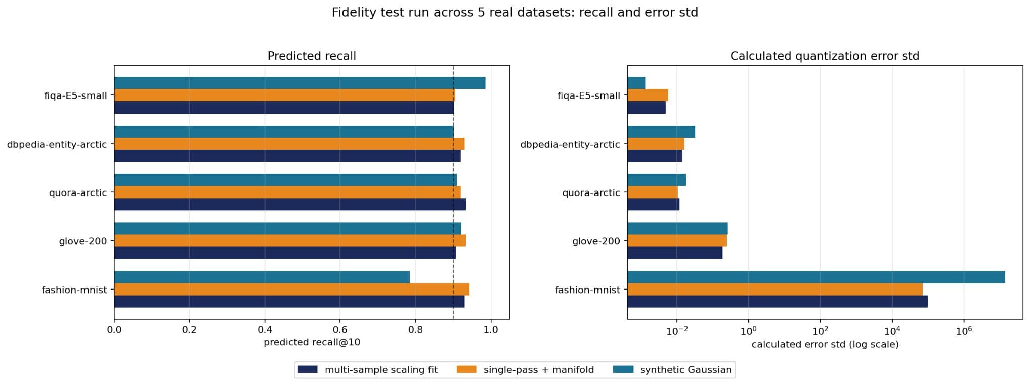
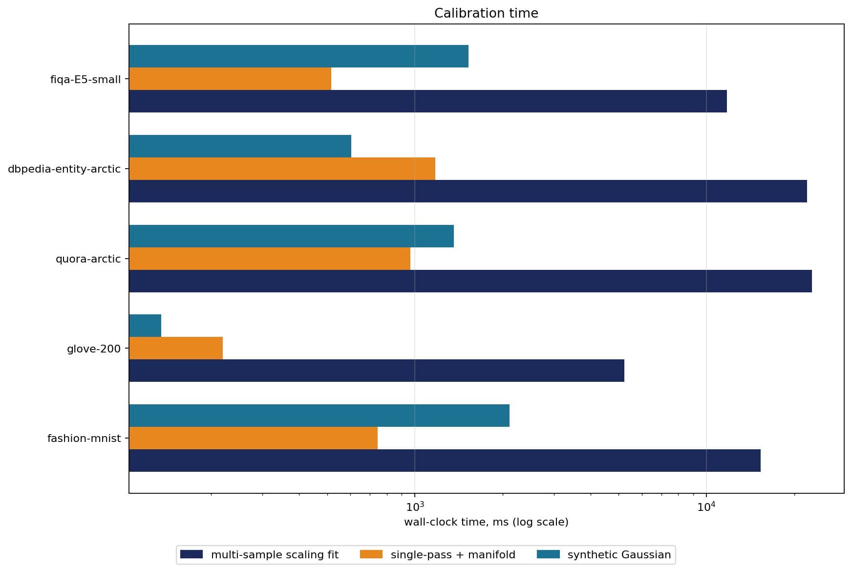
The single-pass real residual measurement's calculated error SD is closer to the multi-sample scaling fit (our gold standard), with respect to the synthetic Gaussian residuals. Consequently, the predicted recall is closer when using the single-pass + manifold plugin method. Indeed, we found the models to be essentially interchangeable regarding the indexing decisions they lead to. Critically, we lower the calibration overhead by an order of magnitude.
Auto calibration overhead on indexing performance
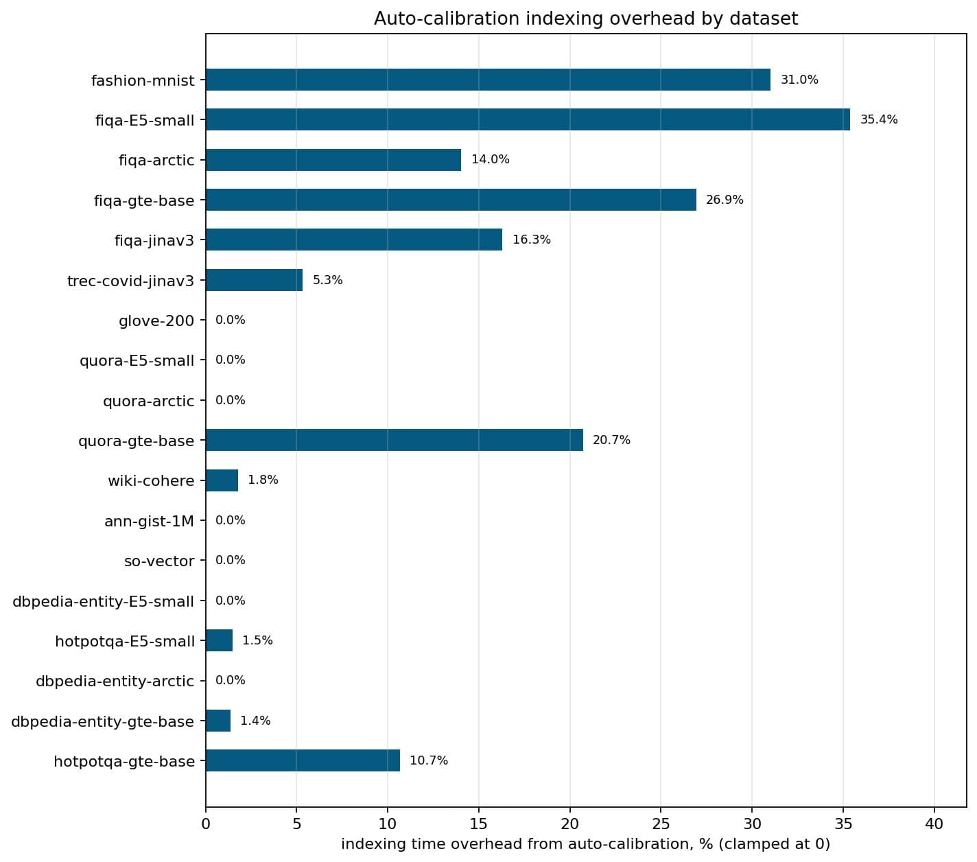
We compared the cost of auto calibration on indexing, when compared with ES defaults, over 18 public benchmarks. We noticed that more than 50% of the datasets report an auto calibration overhead below 2%. Three datasets report 16-27% overhead, while two datasets sit in the 31-35% overhead.
The merge overhead is larger for smaller datasets (Fashion-MNIST, FiQA) that get indexed in a few seconds; that is expected as the size of the vector samples being used for calibration is fixed and therefore more noticeable with tiny datasets. In fact, for larger datasets like DBPedia-Entity and HotpotQA (5M doc vectors) the overhead is sometimes not noticeable and within 11% in the worst case.
What quantization parameters does auto calibration choose?
Looking at the encoding auto-calibration landed on for each of the real datasets:
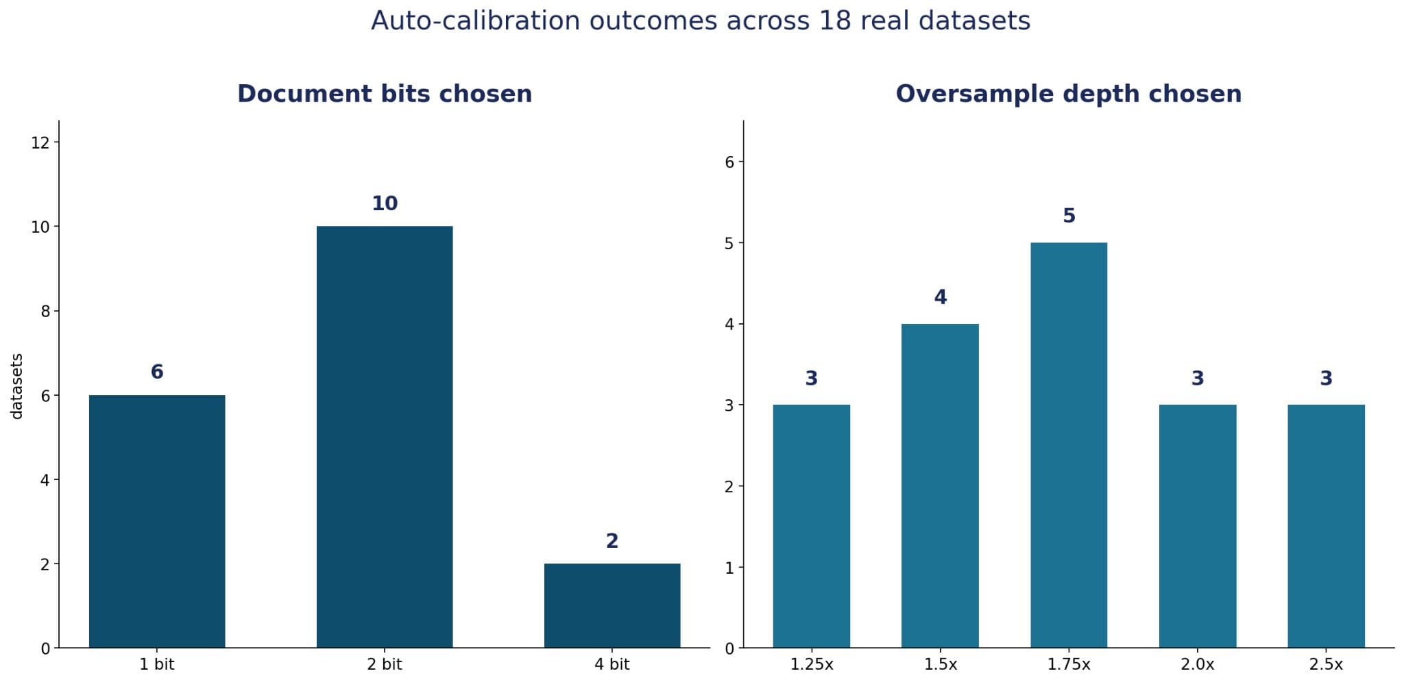
Query bits were 4 in every dataset. While query bits aren't priced into the cost formula, we still iterate through lower query bits first (e.g., at 1 bit doc vectors, we first evaluate recall for 1 bit query vectors, then for 4 bit query vectors); so it’s possible for some datasets to even choose symmetric 1-bit quantization. The center of mass is a 2-bit document encoding with somewhere between 1.5x and 1.75x oversampling; 4-bit only shows up for two genuinely harder datasets (Fashion-MNIST's image embeddings, GIST-1M), and 1-bit only for a handful of the text-embedding models that are most robust to quantization. In fact, our own models are among those that quantize best: we selected 1 bit documents for all three corpuses we tested with Jina v3.
Recall and QPS improvements from automatic calibration
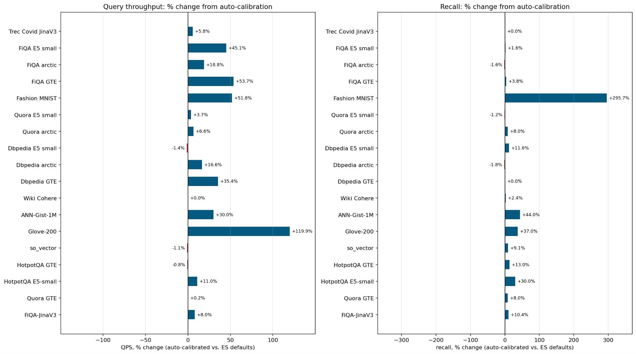
Auto-calibration is a broad win across the eighteen datasets: QPS improves in 15 of 18 cases (often substantially, double digits on about ten, and over +50% on FiQA GTE, Fashion MNIST, and Glove-200), and recall improves in 15 of 18 cases too, including a dramatic +295.7% rescue on Fashion MNIST. Most datasets see gains on both metrics simultaneously, and even the more modest cases still land solidly positive, recall improvements are commonly in the high single digits to double digits, QPS gains follow a similar pattern. Where either metric does dip, the drops are small and contained: the three QPS regressions all stay under 1.5%, and the three recall regressions all stay under 2%.
How to enable auto-calibrated vector quantization in Elasticsearch
The feature is not enabled by default for now, and opt-in via auto_calibrate on bbq_disk index options:
With this set, you no longer need to guess at bits, oversampling, or preconditioning: each segment picks the cheapest configuration that's predicted to hit 90% recall@10 for its own vector distribution, and re-evaluates that choice every time it's merged.
What's next for automatic vector quantization in Elasticsearch
Our first post showed that recall could be predicted in closed form from a small sample. Turning that into something running inside a real merge path meant a second round of engineering decisions that the model itself doesn't answer: how to order a sweep over candidates so it's cheap in the common case, how to price oversampling against document bits given how each is actually paid for at query time, and how to estimate the error term itself cheaply without quietly wrecking its accuracy.
In the end, we have a feature that allows us to tailor indexing choices to the data characteristics, with less than 11% overhead to index time for large indices. This gives us the ability to accurately control recall while optimizing quantization and oversampling choices for query performance. We got an average increase of 16.7% in QPS when we enabled this feature compared to our previous default settings for DiskBBQ. All while reliably achieving our target recall. Taking away the configuration burden from the user actually allows us to make better choices; it is a win-win.
This is the beginning of a longer journey that we’re working on to bring automatic configuration based on a combination of better understanding of the operating environment and better understanding of the data characteristics. We look forward to sharing more of this work with you in the near future.
Contenido relacionado

56% faster, up to 50% better retrieval performance: What's inside Jina's new 600 million parameter listwise reranker
Jina Reranker 3.5 beats v3 by 50%+ on case law, closes the gap with models 7x its size on legal, medical, and financial benchmarks, and beats them outright on structured data. It's a drop-in replacement for v3, with no API changes.
16 de julio de 2026
A picture is worth 1.5x the words: What we learned benchmarking product search embeddings
We benchmarked two embedding models on 5,000 real products and found that combining image and text beats either alone by up to 50%. Here's the data and the model that won.