Seamlessly connect with leading AI and machine learning platforms. Start a free cloud trial to explore Elastic’s gen AI capabilities or try it on your machine now.
Introduction
We talked before about the scalar quantization work we've been doing in Lucene. In this two part blog we will dig a little deeper into how we're optimizing scalar quantization for the vector database use case. This has allowed us to unlock very nice performance gains for int4 quantization in Lucene, as we'll discuss in the second part. In the first part we're going to dive into the details of how we did this. Feel free to jump ahead to learn about what this will actually mean for you. Otherwise, buckle your seatbelts, because Kansas is going bye-bye!
Scalar quantization recap
First of all, a quick refresher on scalar quantization.
Scalar quantization was introduced as a mechanism for accelerating inference. To date it has been mainly studied in that setting. For that reason, the main considerations were the accuracy of the model output and the performance gains that come from reduced memory pressure and accelerated matrix multiplication (GEMM) operations. Vector retrieval has some slightly different characteristics which we can exploit to improve quantization accuracy for a given compression ratio.
The basic idea of scalar quantization is to truncate and scale each floating point component of a vector (or tensor) so it can be represented by an integer. Formally, if you use bits to represent a vector component as an integer in the interval you transform it as follows
where denotes and denotes round to the nearest integer. People typically choose and based on percentiles of the distribution. We will discuss a better approach later.
If you use int4 or 4 bit quantization then each component is some integer in the interval [0,15], that is each component takes one of only 16 distinct values!
Novelties introduced to scalar quantization
In this part, we are going to describe in detail two specific novelties we have introduced:
- A first order correction to the dot product when it is computed using integer values.
- An optimization procedure for the free parameters used to compute the quantized vector.
Just to pause on point 1 for a second. What we will show is that we can continue to compute the dot product directly using integer arithmetic. At the same time, we can compute an additive correction that allows us to improve its accuracy. So we can improve retrieval quality without losing the opportunity of using extremely optimized implementations of the integer dot product. This translates to a clear cut win in terms of retrieval quality as a function of performance.
1. Error correcting the scalar dot product
Most embedding models use either cosine or dot product similarity. The good thing is if you normalize your vectors then cosine (and even Euclidean) is equivalent to dot product (up to order). Therefore, reducing the quantization error in the dot product covers the great majority of use cases. This will be our focus.
The vector database use case is as follows. There is a large collection of floating point vectors from some black box embedding model. We want a quantization scheme which achieves the best possible recall when retrieving with query vectors which come from a similar distribution. Recall is the proportion of true nearest neighbors, those with maximum dot product computed with float vectors, which we retrieve computing similarity with quantized vectors. We assume we've been given the truncation interval for now. All vector components are snapped into this interval in order to compute their quantized values exactly as we discussed before. In the next part we will discuss how to optimize this interval for the vector database use case.
To movitate the following analysis, consider that for any given document vector, if we knew the query vector ahead of time , we could compute the quantization error in the dot product exactly and simply subtract it. Clearly, this is not realistic since, apart from anything else, the query vector is not fixed. However, maybe we can achieve a real improvement by assuming that the query vector is drawn from a distribution that is centered around the document vector. This is plausible since queries that match a document are likely to be in the vicinity of its embedding. In the following, we formalize this intuition and actually derive a correction term. We first study the error that scalar quantization introduces into the dot product. We then devise a correction based on the expected first order error in the vicinity of each indexed vector. To do this requires us to store one extra float per vector. Since realistic vector dimensions are large this results in minimal overhead.
We will call an arbitrary vector in our database and an arbitrary query vector . Then
On the right hand side, the first term is a constant and the second two terms are a function of a single vector and can be precomputed. For the one involving the document, this is an extra float that can be stored with its vector representation. So far all our calculations can use floating point arithmetic. Everything interesting however is happening in the last term, which depends on the interaction between the query and the document. We just need one more bit more notation: define and where we understand that the clamp function broadcasts over vector components. Let's rewrite the last term, still keeping everything in floating point, using a similar trick:
Here, represents the quantization error. The first term is just the scaled quantized vector dot product and can be computed exactly. The last term is proportional in magnitude to the square of the quantization error and we hope this will be somewhat small compared to the overall dot product. That leaves us with the terms that are linear in the quantization error.
We can compute the quantization error vectors in the query and document, and respectively, ahead of time. However, we don't actually know the value of we will be comparing to a given and vice versa. So we don't know how to calculate the error in the dot product quantities exactly. In such cases it is natural to try and minimize the error in expectation (in some sense we discuss below).
If and are drawn at random from our corpus they are random variables and so too are and . For any distribution we average over for then , since and are fixed for a query. This is a constant additive term to the score of each document, which means it does not change their order. This is important as it will not change the quality of retrieval and so we can drop it altogether.
What about the term? The naive thing is to assume that the is a random sample from our corpus. However, this is not the best assumption. In practice, we know that the queries which actually match a document will come from some region in the vicinity of its embedding as we illustrate in the figure below.

Schematic query distribution that is expected to match a given document embedding (orange) vs all queries (blue plus orange).
We can efficiently find nearest neighbors of each document in the database once we have a proximity graph. However, we can do something even simpler and assume that for relevant queries . This yields a scalar correction which only depends on the document embedding and can be precomputed and added on to the term and stored with the vector. We show later how this affects the quality of retrieval. The anisotropic correction is inspired by this approach for reducing product quantization errors.
Finally, we note that the main obstacle to improving this correction is we don't have useful estimates of the joint distribution of the query and document embedding quantization errors. One approach that might enable this, at the cost of some extra memory and compute, is to use low rank approximations of these errors. We plan to study schemes like this since we believe they could unlock accurate general purpose 2 or even 1 bit scalar quantization.
2. Optimizing the truncation interval
So far we worked with some specified interval but didn't discuss how to compute it. In the context of quantization for model inference people tend to use quantile points of the component distribution or their minimum and maximum. Here, we discuss a new method for computing this based on the idea that preserving the order of the dot product values is better suited to the vector database use case.
First off, why is this not equivalent to minimizing the magnitude of the quantization errors? Suppose for a query the top-k matches are for . Consider two possibilities, the quantization error is some constant , or it is is normally distributed with mean and standard deviation . In the second case the expected error is roughly 10 times smaller than the first. However, the first effect is a constant shift, which preserves order and has no impact on recall. Meanwhile, if it is very likely the random error will reorder matches and so affect the quality of retrieval.
Let's use the previous example to better motivate our approach. The figure below shows the various quantities at play for a sample query and two documents and . The area of each blue shaded rectangle is equal to one of the floating point dot products and the area of each red shaded rectangle is equal to one of the quantization errors. Specifically, the dot products are and , and the quantization errors are and where is the projection onto the query vector. In this example the errors preserve the document order. This follows because the right blue rectangle (representing the exact dot product) and union of right blue and red rectangles (representing the quantized dot product) are both larger than the left ones. It is visually clear the more similar the left and right red rectangles the less likely it is the documents will be reordered. Conversely, the more similar the left and right blue rectangles the more likely it is that quantization will reorder them.

Schematic of the dot product values and quantization error values for a query and two near neighbor documents. In this case, the document order is preserved by quantization.
One way to think of the quantized dot product is that it models the floating point dot product. From the previous discussion we want to minimize the variance of this model's residual error, which should be as similar as possible for each document. However, there is a second consideration: the density of the floating point dot product values. If these values are close together it is much more likely that quantization will reorder them. It is quite possible for this density to change from one part of the embedding space to another and higher density regions are more sensitive to quantization errors.
A natural measure which captures both the quantization error variance and the density of the dot product values is the coefficient of determination of the quantized dot product with respect to the floating point dot product. A good interval will maximize this in expectation over a representative query distribution. We need a reasonable estimator for this quantity for the database as a whole that we can compute efficiently. We found the following recipe is both fast and yields an excellent choice for parameters and :
- Sample 1000 random document vectors from the index.
- For each sample vector find its 10 nearest neighbors.
- Maximize the average coefficient of determination of the quantized dot product between the sampled vectors and their nearest neighbors with respect to the interval .
This optimization problem can be solved by any black box solver. For example, we used a variant of the adaptive LIPO algorithm in the following. Furthermore, we found that our optimization objective was well behaved (low Lipschitz constant) for all data sets we tested.
Proof of principle for int4 quantization
Before deciding to implement this scheme for real we studied how it behaves with int4 quantization.
Below we show results for two data sets that are fairly typical of passage embedding model distributions on real data. To generate these we use e5-small-v2 and Cohere's multilingual-22-12 models. These are both fairly state-of-the-art text embedding models. However, they have rather different characteristics. The e5-small-v2 model uses cosine similarity, its vectors have 384 dimensions and very low angular variation. The multilingual-22-12 model uses dot product similarity, its vectors have 768 dimensions and it encodes information in their length. They pose rather different challenges for our quantization scheme and improving both gives much more confidence it works generally. For e5-small-v2 we embedded around 500K passages and 10K queries sampled from the MS MARCO passage data set. For multilingual-22-12 we used around 1M passages and 1K distinct passages for queries sampled from the English Wikipedia data set.
First of all, it is interesting to understand the accuracy of the int4 dot product values. The figure below shows the int4 dot product values compared to their float values for a random sample of 100 documents and their 10 nearest neighbors taken from the set we use to compute the optimal truncation interval for e5-small-v2. The orange “best fit” line is . Note that this underlines the fact that this procedure can pick a biased estimator if it reduces the residual variance: in this case the quantized dot product is systematically underestimating the true dot product. However, as we discussed before, any constant shift in the dot product is irrelevant for ranking. For the full 1k samples we achieve an of a little less than 0.995, i.e. the int4 quantized dot product is a very good model of the float dot product!

Comparison of int4 dot product values to the corresponding float values for a random sample of 100 documents and their 10 nearest neighbors.
While this is reassuring, what we really care about is the impact on retrieval quality. Since one can implement brute force nearest neighbor search in a few lines, it allows us to quickly test the impact of our design choices on retrieval. In particular, we are interested in understanding the expected proportion of true nearest neighbors we retrieve when computing similarities using int4 quantized vectors. Below we show the results for an ablation study of the dot product correction and interval optimization.
In general, one can boost the accuracy of any quantization scheme by gathering more than the requested vector count and reranking them using their floating point values. However, this comes with a cost: it is significantly more expensive to search graphs for more matches and the floating point vectors must be loaded from disk or it defeats the purpose of compressing them. One way of comparing alternatives is therefore to understand how many vectors must be reranked to achieve the same recall. The lower this number is, the better. In the figures below we show average recall curves as a function of the number of candidates we rerank for different combinations of the two improvements we have discussed:
- “Baseline” sets to the central confidence and applies no correction to the dot product,
- “No correction” optimizes the interval by maximizing but applies no correction to the dot product,
- “No optimization” sets to the central confidence but applies the linear correction to the dot product, and
- “Our scheme” optimizes the interval by maximizing and applies the linear correction to the dot product.
Note that we used to denote the vector dimension.

Average recall@10 curves for e5-small-v2 embeddings as a function of the number of candidates reranked for different combinations of the two improvements we discussed.

Average recall@10 curves for multilingual-22-12 embeddings as a function of the number of candidates reranked for different combinations of the two improvements we discussed.
For e5-small-v2 embeddings we roughly halve the number of vectors we need to rerank to achieve 95% recall compared to the baseline. For multilingual-22-12 embeddings we reduce it by closer to a factor of three. Interestingly, the impact of the two improvements is different for the different data sets. For e5-small-v2 embeddings applying the linear correction has a significantly larger effect than optimizing the interval whilst the converse is true for multilingual-22-12 embeddings. Another important observation is the gains are more significant if one wants to achieve very high recall: to achieve close to 99% recall one has to rerank at least 5 times as many vectors for both data sets in the baseline versus our improved quantization scheme.
Conclusion
We have discussed the theoretical and empirical motivation behind two novelties we introduced to achieve high quality int4 quantization, as well as some preliminary results that indicate it'll be an effective general purpose scheme for in memory vector storage for retrieval. This is all well and good, but how well does it work in a real vector database implementation? In the companion blog we discuss our implementation in Lucene and compare it to other storage options such as floating point and int7, which Lucene also provides.
Related Content
July 13, 2026
The disk that never woke up: what actually decided our Qdrant vector search benchmark rematch
On the same hardware, Elasticsearch and Qdrant land in the same range at 56 QPS. The io_uring disk scorer and memory claims turned out to be the two things that mattered least.
July 10, 2026
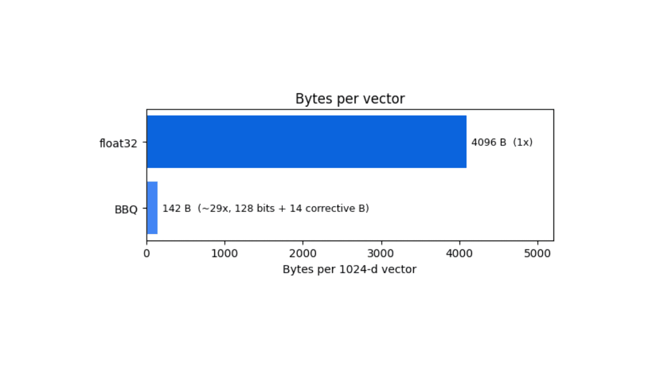
How BBQ shrinks Jina v5 embeddings by 29x without losing recall in Elasticsearch
A hands-on test comparing BBQ and float32 vector indices in Elasticsearch, measuring memory, disk and recall@10 across five languages.
July 7, 2026
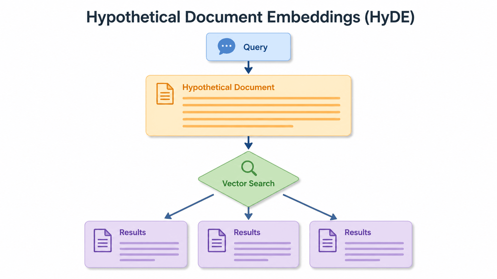
Short queries, formal documents: how HyDE improved semantic search precision by 50% in Elasticsearch
HyDE boosts semantic search precision and recall by 50% on short queries. Here's how to implement it in Elasticsearch with the Inference API and semantic_text.
July 2, 2026
A simdvec deep-dive: How Elasticsearch uses neural-net and video-codec CPU instructions for vector search
Four ways Elasticsearch's vector search engine reuses neural-network, video-codec and cryptography CPU instructions for up to 6x speedups; with the math, the failed attempts and the benchmarks.
June 24, 2026
Elasticsearch DiskBBQ delivers 7x faster vector search than Qdrant on network-attached storage
Elasticsearch DiskBBQ achieves up to 7x higher vector search throughput than Qdrant at comparable recall on network-attached storage. Explore the benchmark methodology and full results.