Want to get Elastic certified? Find out when the next Elasticsearch Engineer training is running! You can start a free cloud trial or try Elastic on your local machine now.
Introduction to Int4 quantization in Lucene
In our previous blogs, we walked through the implementation of scalar quantization as a whole in Lucene. We also explored two specific optimizations for quantization. Now we've reached the question: how does int4 quantization work in Lucene and how does it line up?
How does
Storing and scoring the quantized vectors
Lucene stores all the vectors in a flat file, making it possible for each vector to be retrieved given some ordinal. You can read a brief overview of this in our previous scalar quantization blog.
Nowint4 gives us additional compression options than what we had before. It reduces the quantization space to only 16 possible values (0 through 15). For more compact storage, Lucene uses some simple bit shift operations to pack these smaller values into a single byte, allowing a possible 2x space savings on top of the already 4x space savings with int8. In all, storing int4 with bit compression is 8x smaller than float32.

Figure 1: This shows the reduction in bytes required with int4 which allows an 8x reduction in size from float32 when compressed.
int4 also has some benefits when it comes to scoring latency. Since the values are known to be between 0-15, we can take advantage of knowing exactly when to worry about value overflow and optimize the dot-product calculation. The maximum value for a dot product is 15*15=225 which can fit in a single byte. ARM processors (like my macbook) have a SIMD instruction length of 128 bits (16 bytes). This means that for a Java short we can allocate 8 values to fill the lanes. For 1024 dimensions, each lane will end up accumulating a total of 1024/8=128 multiplications that have a max value of 225. The resulting maximum sum of 28800 fits well within the limit of Java's short value and we can iterate more values at a time than. Here is some simplified code of what this looks like for ARM.
Calculating the quantization error correction
For a more detailed explanation of the error correction calculation and its derivation, please see error correcting the scalar dot-product.
Here is a short summary, woefully (or joyfully) devoid of complicated mathematics.
For every quantized vector stored, we additionally keep track of a quantization error correction. Back in the Scalar Quantization 101 blog there was a particular constant mentioned:
This constant is a simple constant derived from basic algebra. However, we now include additional information in the stored float that relates to the rounding loss.
Where is each floating point vector dimension, is the scalar quantized floating point value, and .
This has two consequences. The first is intuitive, as it means that for a given set of quantization buckets, we are slightly more accurate as we account for some of the lossiness of the quantization. The second consequence is a bit more nuanced. It now means we have an error correction measure that is impacted by the quantization bucketing. This implies that it can be optimized.
Finding the optimal bucketing for int4 quantization
The naive and simple way to do scalar quantization can get you pretty far. Usually, you pick a confidence interval from which you calculate the allowed extreme boundaries for vector values. The default in Lucene and consequently Elasticsearch is . Figure 2 shows the confidence interval over some sampled CohereV3 embeddings. Figure 3 shows the same vectors, but scalar quantized with that statically set confidence interval.

Figure 2: A sampling of CohereV3 dimension values.

Figure 3: CohereV3 dimension values quantized into int7 values. What are those spikes at the end? Well, that is the result of truncating extreme values during the quantization process.
But, we are leaving some nice optimizations on the floor. What if we could tweak the confidence interval to shift the buckets, allowing for more important dimensional values to have higher fidelity. To optimize, Lucene does the following:
- Sample around 1,000 vectors from the data set and calculate their true nearest 10 neighbors.
- Calculate a set of candidate upper and lower quantiles. The set is calculated by using two different confidence intervals: and . These intervals are on the opposite extremes. For example, vectors with
1024dimensions would search quantile candidates between confidence intervals0.99902and0.90009. - Do a grid search over a subset of the quantiles that exist between these two confidence intervals. The grid search finds the quantiles that maximize the coefficient of determination of the quantization score errors vs. the true 10 nearest neighbors calculated earlier.

Figure 3: Lucene searching the confidence interval space and testing various buckets for int4 quantization.

Figure 4: The best int4 quantization buckets found for this CohereV3 sample set.
For a more complete explanation of the optimization process and the mathematics behind this optimization, see optimizing the truncation interval.
Speed vs. size for quantization
As I mentioned before, int4 gives you an interesting tradeoff between performance and space. To drive this point home, here are some memory requirements for CohereV3 500k vectors.

Figure 5: Memory requirements for CohereV3 500k vectors.
Of course, we see the typical 4x reduction in regular scalar quantization, but then additional 2x reduction with int4. Moving the required memory from 2GB to less than 300MB. Keep in mind, this is with compression enabled. Decompressing and compressing bytes does have an overhead at search time. For every byte vector, we must decompress them before doing the int4 comparisons. Consequently, when this is introduced in Elasticsearch, we want to give users the ability to choose to compress or not. For some users, the cheaper memory requirements are just too good to pass up, for others, their focus is speed. Int4 gives the opportunity to tune your settings to fit your use-case.

Figure 6: HNSW graph search speed comparison for CohereV3 500k vectors.
Speed part 2: more SIMD in int4
Figure 6 is a bit disappointing in terms of the speed of compressed scalar quantization. We expect performance benefits from loading fewer bytes to the JVM heap. However, this is being outweighed by the cost of decompressing them. This caused us dig deeper. The reason for the performance impact was naively decompressing the bytes separately from the dot-product comparison. This is a mistake. We can do better.
Consequently, we can use SIMD to decompress the bytes and compare them in the same function. This is a bit more complicated than the previous SIMD example, but it is possible. Here is a simplified version of what this looks like for ARM.
As expected, this has a significant improvement on ARM. Effectively removing all performance discrepancies on ARM between compressed and uncompressed scalar quantization.

Figure 7: HNSW graph search comparison with int4 quantized vectors over 500k Coherev3 vectors. This is on ARM architecture.
The end?
Over the last two large and technical blog posts, we've gone over the math and intuition around the optimizations and what they bring to Lucene. It's been a long ride, and we are nowhere near done. Keep an eye out for these capabilities in a future Elasticsearch version!
Frequently Asked Questions
What is Int4 quantization in Lucene?
Int4 provides additional compression options. It reduces the quantization space to only 16 possible values (0 through 15).
Related Content
July 10, 2026
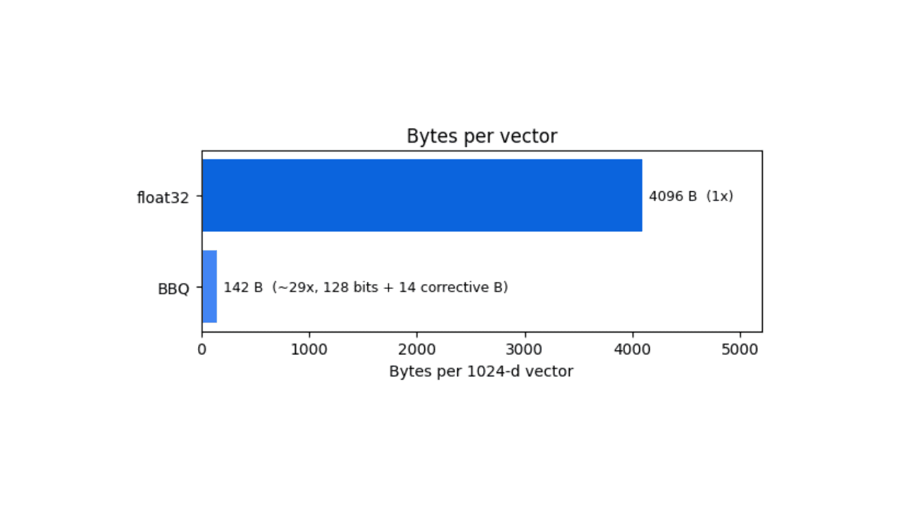
How BBQ shrinks Jina v5 embeddings by 29x without losing recall in Elasticsearch
A hands-on test comparing BBQ and float32 vector indices in Elasticsearch, measuring memory, disk and recall@10 across five languages.
July 21, 2026
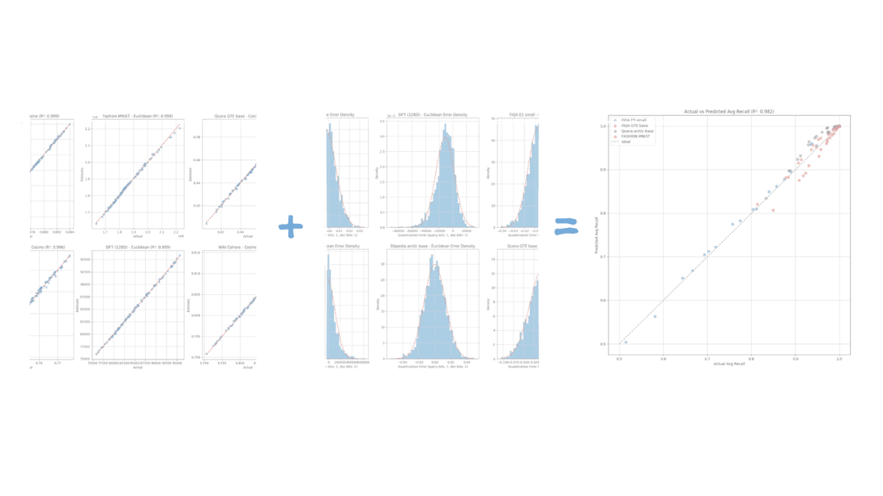
How Elasticsearch auto-tunes vector quantization to hit your recall target
Learn the geometric model that lets Elasticsearch predict recall with R² > 0.98 accuracy and auto-select vector quantization parameters from a small data sample.

June 29, 2026
Bringing it together: How we rebuilt Elasticsearch as a columnar metrics engine; 6.6x less storage, 160x faster queries
Elasticsearch metrics in version 9.4 run on a fully columnar engine: 6.6x less storage, 160x faster queries, native PromQL and OTel support.
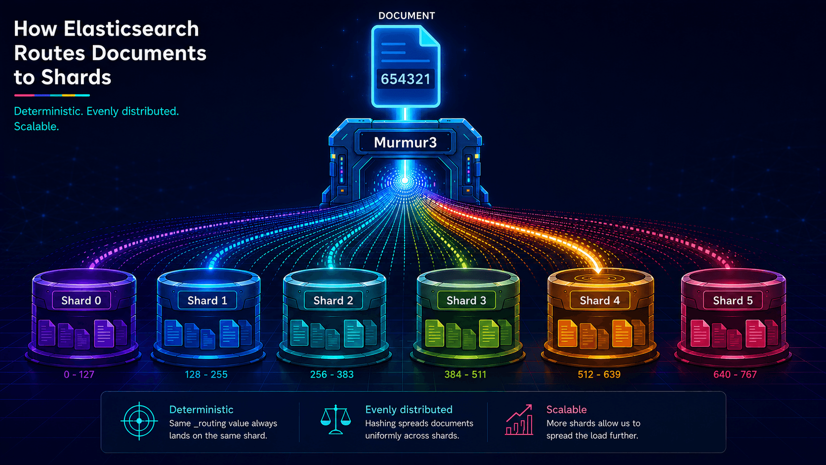
The hash() Elasticsearch won't name and the 12 bytes that prove it's Murmur3
Elasticsearch's routing formula uses MurmurHash3, but the docs never say so. This post names the function, walks through the full shard calculation, and shows you how to reproduce it externally.
June 24, 2026
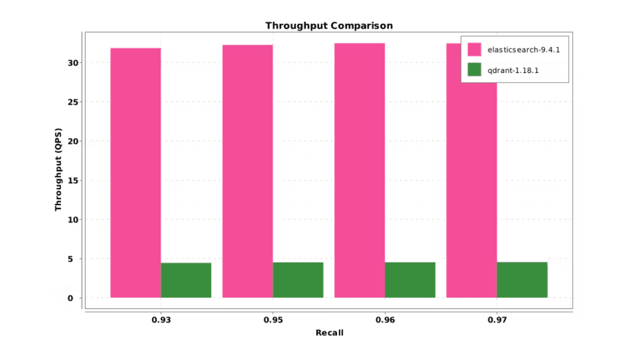
Elasticsearch DiskBBQ delivers 7x faster vector search than Qdrant on network-attached storage
Elasticsearch DiskBBQ achieves up to 7x higher vector search throughput than Qdrant at comparable recall on network-attached storage. Explore the benchmark methodology and full results.