Seamlessly connect with leading AI and machine learning platforms. Start a free cloud trial to explore Elastic’s gen AI capabilities or try it on your machine now.
In this blog, we discuss the work we've been doing to augment Elastic's out-of-the-box retrieval with a pre-trained language model: the Elastic Learned Sparse Encoder (ELSER).
In our previous blog post in this series, we discussed some of the challenges applying dense models to retrieval in a zero-shot setting. This is well known and was highlighted by the BEIR benchmark, which assembled diverse retrieval tasks as a proxy to the performance one might expect from a model applied to an unseen data set. Good retrieval in a zero-shot setting is exactly what we want to achieve, namely a one-click experience that enables textual fields to be searched using a pre-trained model.
This new capability fits into the Elasticsearch _search endpoint as just another query clause, a text_expansion query. This is attractive because it allows search engineers to continue to tune queries with all the tools Elasticsearch already provides. Furthermore, to truly achieve a one-click experience, we've integrated it with the new Elasticsearch Relevance Engine. However, rather than focus on the integration, this blog digs a little into ELSER's model architecture and the work we did to train it.
We had another goal at the outset of this project. The natural language processing (NLP) field is fast moving, and new architectures and training methodologies are being introduced rapidly. While some of our users will keep on top of the latest developments and want full control over the models they deploy, others simply want to consume a high quality search product. By developing our own training pipeline, we have a playground for implementing and evaluating the latest ideas, such as new retrieval relevant pre-training tasks or more effective distillation tasks, and making the best ones available to our users.
Finally, it is worth mentioning that we view this feature as complementary to the existing model deployment and vector search capabilities in the Elastic Stack, which are needed for those more custom use cases like cross-modal retrieval.
ELSER performance results
Before looking at some of the details of the architecture and how we trained our model, the Elastic Learned Sparse Encoder (ELSER), it's interesting to review the results we get, as ultimately the proof of the pudding is in the eating.
As we discussed before, we use a subset of BEIR to evaluate our performance. While this is by no means perfect, and won't necessarily represent how the model behaves on your own data, we at least found it challenging to make significant improvements on this benchmark. So we feel confident that improvements we get on this translate to real improvements in the model. Since absolute performance numbers on benchmarks by themselves aren't particularly informative, it is nice to be able to compare with other strong baselines, which we do below.
The table below shows the performance of Elastic Learned Sparse Encoder compared to Elasticsearch's BM25 with an English analyzer broken down by the 12 data sets we evaluated. We have 10 wins, 1 draw, and 1 loss and an average improvement in NDCG@10 of 17%.

NDCG@10 for BEIR data sets for BM25 and Elastic Learned Sparse Encoder (referred to as “ELSER” above, note higher is better)
In the following table, we compare our average performance to some other strong baselines. The Vespa results are based on a linear combination of BM25 and their implementation of ColBERT as reported here, the Instructor results are from this paper, the SPLADEv2 results are taken from this paper and the OpenAI results are reported here. Note that we've separated out the OpenAI results because they use a different subset of the BEIR suite. Specifically, they average over ArguAna, Climate FEVER, DBPedia, FEVER, FiQA, HotpotQA, NFCorpus, QuoraRetrieval, SciFact, TREC COVID and Touche. If you follow that link, you will notice they also report NDCG@10 expressed as a percentage. We refer the reader to the links above for more information on these approaches.

Average NDCG@10 for BEIR data sets vs. various high quality baselines (higher is better). Note: OpenAI chose a different subset, and we report our results on this set separately.
Finally, we note it has been widely observed that an ensemble of statistical (a la BM25) and model based retrieval, or hybrid search, tends to outperform either in a zero-shot setting. Already in 8.8, Elastic allows one to do this for text_expansion with linear boosting and this works well if you calibrate to your data set. We are also working on Reciprocal Rank Fusion (RRF), which performs well without calibration. Stay tuned for our next blog in this series, which will discuss hybrid search.
Having seen how ELSER performs, we next discuss its architecture and some aspects of how it is trained.
What are learned sparse models and why are they attractive?
We showed in our previous blog post that, while very effective if fine-tuned, dense retrieval tends not to perform well in a zero-shot setting. By contrast cross-encoder architectures, which don't scale well for retrieval, tend to learn robust query and document representations and work well on most text. It has been suggested that part of the reason for this difference is the bottleneck of the query and document interacting only via a relatively low dimensional vector “dot product.” Based on this observation, a couple of model architectures have been recently proposed that try to reduce this bottleneck — these are ColBERT and SPLADE.
From our perspective, SPLADE has some additional advantages:
- Compared to ColBERT, it is extremely storage efficient. Indeed, we find that document passages expand to about 100 tokens on average and we've seen approximate size parity with normal text indices.
- With some caveats, retrieval can make use of inverted indices for which we already have very mature implementations in Lucene. Compared to ANN, these use memory extremely efficiently.
- It provides natural controls as it is being trained that allow us to trade retrieval quality for retrieval latency. In particular, the FLOPS regularizer, which we discuss below, allows one to add a term to the loss for the expected retrieval cost. We plan to take advantage of this as we move toward GA.
One last clear advantage compared to dense retrieval is that SPLADE allows one a simple and compute efficient route to highlight words generating a match. This simplifies surfacing relevant passages in long documents and helps users better understand how the retriever is working. Taken together, we felt that these provided a compelling case for adopting the SPLADE architecture for our initial release of this feature.
There are multiple good detailed descriptions of this architecture — if you are interested in diving in, this, for example, is a nice write up by the team that created the model. In very brief outline, the idea is rather than use a distributed representation, say averaging BERT token output embeddings, instead use the token logits, or log-odds the tokens are predicted, for masked word prediction.
When language models are used to predict masked words, they achieve this by predicting a probability distribution over the tokens of their vocabulary. The BERT vocabulary, for WordPiece, contains many common real words such as cat, house, and so on. It also contains common word endings — things like ##ing (with the ## simply denoting it is a continuation). Since words can't be arbitrarily exchanged, relatively few tokens will be predicted for any given mask position. SPLADE takes as a starting point for its representation of a piece of text the tokens most strongly predicted by masking each word of that text. As noted, this is a naturally disentangled or sparse representation of that text.

It is reasonable to think of these token probabilities for word prediction as roughly capturing contextual synonyms. This has led people to view learned sparse representations, such as SPLADE, as something close to automatic synonym expansion of text, and we see this in multiple online explanations of the model.
In our view, this is at best an oversimplification and at worst misleading. SPLADE takes as the starting point for fine-tuning the maximum token logits for a piece of text, but it then trains on a relevance prediction task, which crucially accounts for the interaction between all shared tokens in a query and document. This process somewhat re-entangles the tokens, which start to behave more like components of a vector representation (albeit in a very high dimensional vector space).
We explored this a little as we worked on this project. We saw as we tried removing low score and apparently unrelated tokens in the expansion post hoc that it reduced all quality metrics, including precision(!), in our benchmark suite. This would be explained if they were behaving more like a distributed vector representation, where zeroing individual components is clearly nonsensical. We also observed that we can simply remove large parts of BERT's vocabulary at random and still train highly effective models as the figure below illustrates. In this context, parts of the vocabulary must be being repurposed to account for the missing words.

Margin MSE validation loss for student models with different vocabulary sizes
Finally, we note that unlike say generative tasks where size really does matter a great deal, retrieval doesn't as clearly benefit from having huge models. We saw in the result section that this approach is able to achieve near state-of-the-art performance with only 100M parameters, as compared to hundreds of millions or even billions of parameters in some of the larger generative models. Typical search applications have fairly stringent requirements on query latency and throughput, so this is a real advantage.
Exploring the training design space for ELSER
In our first blog, we introduced some of the ideas around training dense retrieval models. In practice, this is a multi stage process and one typically picks up a model that has already been pre-trained. This pre-training task can be rather important for achieving the best possible results on specific downstream tasks. We don't discuss this further because to date this hasn't been our focus, but note in passing that like many current effective retrieval models, we start from a co-condenser pre-trained model.
There are many potential avenues to explore when designing training pipelines. We explored quite a few, and suffice to say, we found making consistent improvements on our benchmark was challenging. Multiple ideas that looked promising on paper didn't provide compelling improvements. To avoid this blog becoming too long, we first give a quick overview of the key ingredients of the training task and focus on one novelty we introduced, which provided the most significant improvements. Independent of specific ingredients, we also made some qualitative and quantitative observations regarding the role of the FLOPS regularization, which we will discuss at the end.
When training models for retrieval, there are two common paradigms: contrastive approaches and distillation approaches. We adopted the distillation approach because this was shown to be very effective for training SPLADE in this paper. The distillation approach is slightly different from the common paradigm, which informs the name, of shrinking a large model to a small, but almost as accurate, “copy.” Instead the idea is to distill the ranking information present in a cross-encoder architecture. This poses a small technical challenge: since the representation is different, it isn't immediately clear how one should mimic the behavior of the cross-encoder with the model being trained. The standard idea we used is to present both models with triplets of the form (query, relevant document, irrelevant document). The teacher model computes a score margin, namely , and we train the student model to reproduce this score margin using MSE to penalize the errors it makes.
Let's think a little about what this process does since it motivates the training detail we wish to discuss. If we recall that the interaction between a query and document using the SPLADE architecture is computed using the dot product between two sparse vectors, of non-negative weights for each token, then we can think about this operation as wanting to increase the similarity between the query and the higher scored document weight vectors. It is not 100% accurate, but not misleading, to think of this as something like “rotating” the query in the plane spanned by the two documents' weight vectors toward the more relevant one. Over many batches, this process gradually adjusts the weight vectors starting positions so the distances between queries and documents captures the relevance score provided by the teacher model.
This leads to an observation regarding the feasibility of reproducing the teacher scores. In normal distillation, one knows that given enough capacity the student would be able to reduce the training loss to zero. This is not the case for cross-encoder distillation because the student scores are constrained by the properties of a metric space induced by the dot product on their weight vectors. The cross-encoder has no such constraint. It is quite possible that for particular training queries and and documents and we have to simultaneously arrange for to be close to and , and to be close to but far from . This is not necessarily possible, and since we penalize the MSE in the scores, one effect is an arbitrary reweighting of the training triplets associated with these queries and documents by the minimum margin we can achieve.
One of the observations we had while working on training ELSER was the teacher was far from infallible. We initially observed this by manually investigating query-relevant document pairs that were assigned unusually low scores. In the process, we found objectively misscored query-document pairs. Aside from manual intervention in the scoring process, we also decided to explore introducing a better teacher.
Following the literature, we were using MiniLM L-6 from the SBERT family for our initial teacher. While this shows strong performance in multiple settings, there are better teachers, based on their ranking quality. One example is a ranker based on a large generative model: monot5 3b. In the figure below, we compare the query-document score pair distribution of these two models. The monot5 3b distribution is clearly much less uniform, and we found when we tried to train our student model using its raw scores the performance saturated significantly below using MiniLM L-6 as our teacher. As before, we postulated that this was down to many important score differences in the peak around zero getting lost with training worried instead about unfixable problems related to the long lower tail.

Monot5 3b and MiniLM L-6 score distributions on a matched scale for a random sample of query-document pairs from the NQ data set. Note: the X-axis does not show the actual scores returned by either of the models.
It is clear that all rankers are of equivalent quality up to monotonic transforms of their scores. Specifically, it doesn't matter if we use or provided is a monotonic increasing function; any ranking quality measure will be the same. However, not all such functions are equivalently effective teachers. We used this fact to smooth out the distribution of monot5 3b scores, and suddenly our student model trained and started to beat the previous best model. In the end, we used a weighted ensemble of our two teachers.
Before closing out this section, we want to briefly mention the FLOPS regularizer. This is a key ingredient of the improved SPLADE v2 training process. It was proposed in this paper as a means of penalizing a metric directly related to the compute cost for retrieval from an inverted index. In particular, it encourages tokens that provide little information for ranking to be dropped from the query and document representations based on their impact on the cost for retrieving from an inverted index. We had three observations:
- Our first observation was that the great majority of tokens are actually dropped while the regularizer is still warming up. In our training recipe, the regularizer uses quadratic warm up for the first 50,000 batches. This means that in the first 10,000 batches, it is no more than 1/25th its terminal value, and indeed we see that the contribution to the loss from MSE in the score margin is orders of magnitude larger than the regularization loss at this point. However, during this period the number of query and document tokens per batch activated by our training data drops from around 4k and 14k on average to around 50 and 300, respectively. In fact, 99% of all token pruning happens in this phase and seems largely driven by removing tokens which actually hurt ranking performance.
- Our second observation was that we found it contributes to ELSER's generalization performance for retrieval. Both turning down the amount of regularization and substituting regularizers that induce more sparseness, such as the sum of absolute weight values, reduced average ranking performance across our benchmark.
- Our final observation was that larger batches and diverse batches both positively impacted retrieval quality; we tried by contrast query clustering with in-batch negatives.
So why could this be, since it is primarily aimed at optimizing retrieval cost? The FLOPS regularizer is defined as follows: it first averages the weights for each token in the batch across all the queries and separately the documents it contains, it then sums the squares of these average weights. If we consider that the batch typically contains a diverse set of queries and documents, this acts like a penalty that encourages something analogous to stop word removal. Tokens that appear for many distinct queries and documents will dominate the loss, since the contribution from rarely activated tokens is divided by the square of the batch size. We postulate that this is actually helping the model to find better representations for retrieval. From this perspective, the fact that the regularizer term only gets to observe the token weights of queries and documents in the batch is undesirable. This is an area we'd like to revisit.
Conclusion
We have given a brief overview of the model, the Elastic Learned Sparse Encoder (ELSER), its rationale, and some aspects of the training process behind the feature we're releasing in a technical preview for the new text_expansion query and integrating with the new Elasticsearch Relevance Engine. To date, we have focused on retrieval quality in a zero-shot setting and demonstrated good results against a variety of strong baselines. As we move toward GA, we plan to do more work on operationalizing this model and in particular around improving inference and retrieval performance.
Stay tuned for the next blog post in this series, where we'll look at combining various retrieval methods using hybrid retrieval as we continue to explore exciting new retrieval methods using Elasticsearch.
The release and timing of any features or functionality described in this post remain at Elastic's sole discretion. Any features or functionality not currently available may not be delivered on time or at all.
Elastic, Elasticsearch and associated marks are trademarks, logos or registered trademarks of Elasticsearch N.V. in the United States and other countries. All other company and product names are trademarks, logos or registered trademarks of their respective owners.
Related Content
July 10, 2026
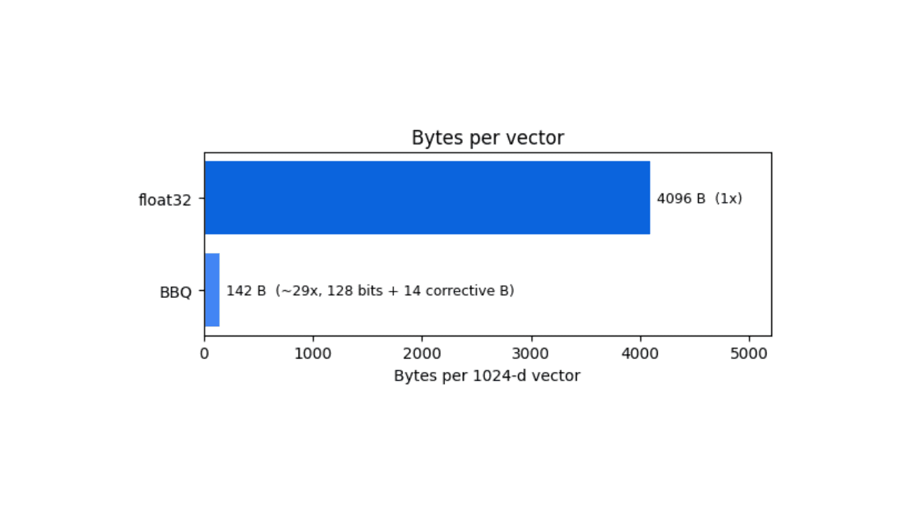
How BBQ shrinks Jina v5 embeddings by 29x without losing recall in Elasticsearch
A hands-on test comparing BBQ and float32 vector indices in Elasticsearch, measuring memory, disk and recall@10 across five languages.
July 7, 2026
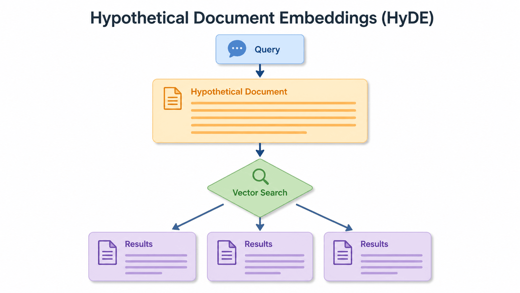
Short queries, formal documents: how HyDE improved semantic search precision by 50% in Elasticsearch
HyDE boosts semantic search precision and recall by 50% on short queries. Here's how to implement it in Elasticsearch with the Inference API and semantic_text.
July 21, 2026
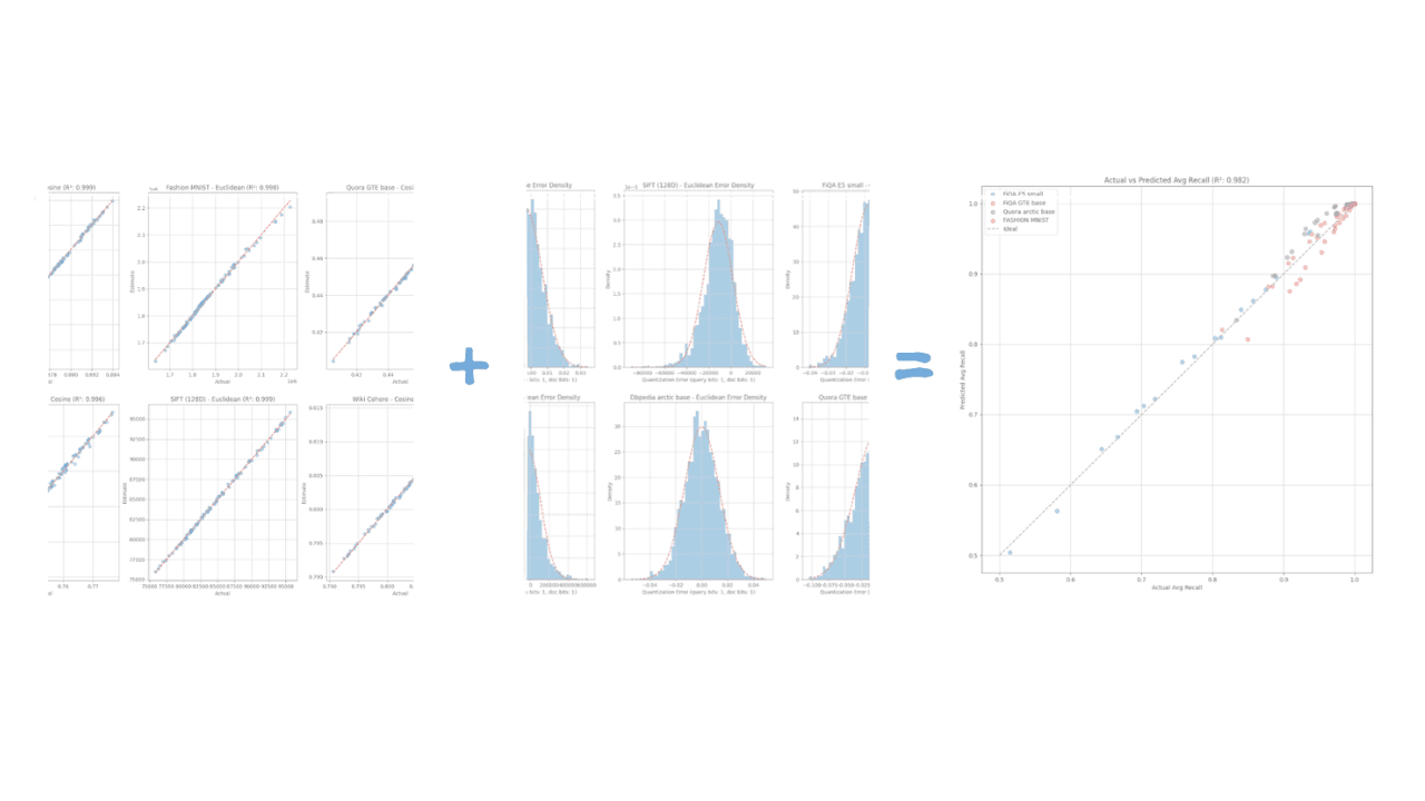
How Elasticsearch auto-tunes vector quantization to hit your recall target
Learn the geometric model that lets Elasticsearch predict recall with R² > 0.98 accuracy and auto-select vector quantization parameters from a small data sample.
June 24, 2026
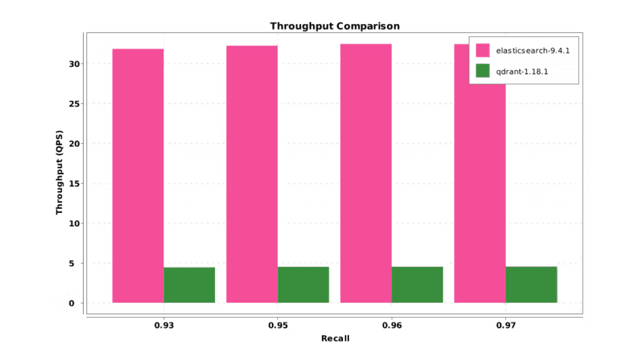
Elasticsearch DiskBBQ delivers 7x faster vector search than Qdrant on network-attached storage
Elasticsearch DiskBBQ achieves up to 7x higher vector search throughput than Qdrant at comparable recall on network-attached storage. Explore the benchmark methodology and full results.
July 24, 2026
How Elasticsearch detects multiple change points in time series with 0.99 recall
ES|QL's CHANGE_POINT command finds structural shifts, variance changes and spikes in any metric in ~1ms, without tuning anything per series.