Elasticsearch is packed with new features to help you build the best search solutions for your use case. Learn how to put them into action in our hands-on webinar on building a modern Search AI experience. You can also start a free cloud trial or try Elastic on your local machine now.
Instrument your search API with about 20 lines of OpenTelemetry (OTel) code, and Elasticsearch Query Language (ES|QL) can tell you what people are searching for, how often they get nothing back, and how fast search actually runs. This builds directly on the first post in this series, where we made the case for using OpenTelemetry over a bespoke analytics pipeline. Here, we wire up a FastAPI search endpoint with custom search.* attributes and run six ES|QL queries against the resulting trace data. On our demo cluster, 17.7% of searches came back empty, a gap we found within minutes of turning the instrumentation on. No separate logging pipeline is required. It's the same spans, attributes, and query language you're probably already running somewhere else in Elastic.
What you'll discover
In this post, you'll learn how to:
- Set up OpenTelemetry in an example Python FastAPI back end.
- Add custom
search.*attributes to your search spans in ~20 lines of code. - Understand how OTel-native ingestion maps attributes to queryable data.
- Write six ES|QL queries against real trace data: top queries, zero-results rate, which queries return nothing, average and max latency, slow query investigation, and search volume over time.
- Turn those queries into saved Kibana visualizations.
What you'll need
- An Elastic Cloud deployment (or self-managed with OTel-native ingestion enabled). Examples tested on Elastic Stack 9.x.
From concept to code: Building the search analytics instrumentation
In the first post, we made the case for using OpenTelemetry to capture search analytics. The idea: Add search.* attributes to your existing OTel spans, send them to Elastic APM, and query them with ES|QL.
Now let's build it.
Want working code? A companion reference project accompanies this series. It's a minimal FastAPI app with the exact instrumentation described below. Clone it, add your Elastic Cloud credentials, and you'll have search analytics data flowing in 10 minutes. Each blog stage maps to a commented-out code block you can enable as you progress.
An OpenTelemetry primer for search API developers
If you've been building search systems but haven't worked with OpenTelemetry before, here's the minimum you need to know.
OTel is an open standard for collecting observability data, traces, metrics, and logs from your applications. It's vendor-neutral: You instrument your code once, and send data to any compatible back end.
The core concept is the span. A span represents a single operation, for example, an API call, a database query, or a search request. Every span has a start time, an end time (the difference is the span duration), and attributes, which are key-value pairs that describe what happened.
Spans nest inside each other to form traces. A trace is a tree of spans that represents one end-to-end request. When a user searches, the trace might look like: browser request → API handler → search logic → Elasticsearch query. Each step is a span, and the parent-child relationships show you exactly where time was spent. This is distributed tracing, which works across services and network boundaries, so a single trace can follow a request from front end to back end to database and back.
Why traces instead of logs? You could log "search query=headphones results=15 took=120ms" and parse it later. But a log line is flat; it can't show you that the 120ms Elasticsearch time sat inside a 250ms API call, revealing 130ms of overhead in your application layer. Traces give you hierarchy, timing, and correlation across services. For search analytics, that means you can see not just what happened but also where time was spent and how operations relate to each other.
For this post, we don't need to understand the full OTel ecosystem. We just need three things:
- Create a span when a search request happens.
- Add attributes to that span, describing the search (such as
search.queryorresult_count). - Send the span to Elastic, where we can query it with ES|QL.
That's it. If you can call span.set_attribute("key", value), you can build search analytics.
What you'll build
By the end of this post, every search request in your API will emit an OTel span that looks like this:
And you'll run six ES|QL queries against real data to answer questions that your team is already asking, using about 20 lines of instrumentation code in total.
Install the OTel SDK
We're using Python and FastAPI here. The same pattern applies to any language with an OTel SDK; the concepts are identical, only the imports change.
Elastic provides the Elastic Distribution of OpenTelemetry Python (EDOT), which bundles the standard OTel SDK with sensible defaults, early access to Elastic-contributed improvements, and a single configure_opentelemetry() call that handles all the boilerplate. We recommend it:
Three packages, two roles:
elastic-opentelemetryEDOT: The OTel API, SDK, and OpenTelemetry Protocol (OTLP) exporter in one package, preconfigured for Elastic.opentelemetry-instrumentation-fastapi: Auto-instruments HTTP endpoints (automatic spans for every request).opentelemetry-instrumentation-elasticsearch: Auto-instruments Elasticsearch client calls (automatic spans for every query).
The auto-instrumentation packages are doing real work here. Without writing a single line of tracing code, you already get HTTP request spans and Elasticsearch query spans. What we're adding is the search-specific context that turns generic traces into analytics.
Using the standard OTel SDK instead? Replace elastic-opentelemetry with opentelemetry-api, opentelemetry-sdk, and opentelemetry-exporter-otlp-proto-http. You'll need to wire up the TracerProvider, OTLPSpanExporter, and BatchSpanProcessor manually (about 10 extra lines). Everything else in this post works the same either way. See the Elastic OTel guide for the full setup.
Configure the connection
OTel uses environment variables for connection configuration. You need four to get started:
| Variable | Purpose | Example |
|---|---|---|
| `OTEL_EXPORTER_OTLP_ENDPOINT` | Managed OTLP (mOTLP) endpoint URL | `https://my-deployment.ingest.us-central1.gcp.elastic-cloud.com` |
| `OTEL_EXPORTER_OTLP_HEADERS` | Authentication | `Authorization=ApiKey <your-api-key>` |
| `OTEL_SERVICE_NAME` | Service name (shown in Kibana APM) | `search-analytics-demo` |
| `OTEL_RESOURCE_ATTRIBUTES` | Other resource attributes | `service.version=1.0.0` |
Where to find these values: In Elastic Cloud, your mOTLP endpoint follows the pattern https://<deployment>.ingest.<region>.gcp.elastic-cloud.com. You can find it in the Elastic Cloud console under your deployment's details or in Kibana at the APM integration page (/app/home#/tutorial/apm) under the OpenTelemetry tab. Your API key can be created from Kibana's Stack Management > API Keys or via the Elasticsearch Create API Key API. For self-managed deployments, you can use the EDOT Collector as an intermediary that receives OTLP and forwards to Elasticsearch.
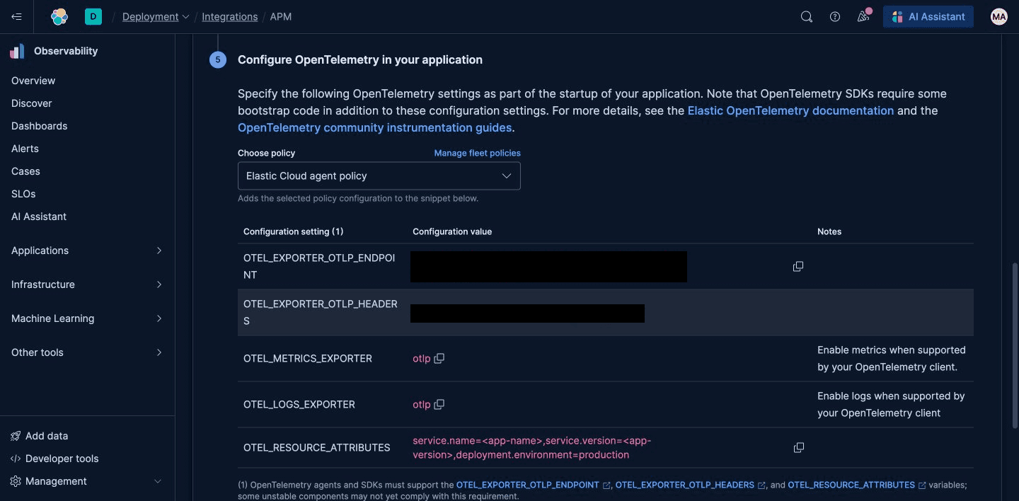
Set them in your environment or .env file:
Initialize the tracer
With EDOT and environment variables configured, initialization wires up three things: the tracer provider and two auto-instrumentation packages that automatically create spans for every HTTP request and every Elasticsearch query:
configure_opentelemetry() reads the OTEL_* environment variables and sets up the tracer provider, exporter, and batch processor with Elastic-optimized defaults, including using the HTTP exporter automatically, which is what the mOTLP endpoint requires. If you see connection errors with vanilla OTel, the most common cause is accidentally using the gRPC exporter instead of HTTP.
The two instrumentors patch the FastAPI and elasticsearch-py libraries at startup so every request and every Elasticsearch call automatically generates a span, without any code changes to individual endpoints.
Instrument your search API
Here's where it gets interesting. This is the code that turns a generic API endpoint into a search analytics source:
A few things worth unpacking.
start_as_current_spancreates the span and sets it as the active span in the current context. This matters because the Elasticsearch client instrumentation picks up the active span and nests its own spans underneath it. You get a span hierarchy automatically.search.query_idis derived from the trace ID. Every trace already has a unique identifier, and we're reusing it as the query identifier. There’s no UUID generation or database sequence. When we add click tracking later, clicks will reference this samequery_idto link back to the search that produced the results.search.result_countdoes double duty. It tells you how many results came back, and when it's zero, you know you have a content gap. There’s no need for a separate boolean flag: Just filter onresult_count == 0in your queries.
Note that the application name is no longer set as a span attribute; it's the service.name resource attribute, configured once via OTEL_SERVICE_NAME. This is the standard OTel approach: Resource attributes describe the service, and span attributes describe the operation.
Normalize search queries before analyzing them
Notice that we're storing request.query as is. That means "Laptop Bag", "laptop bag", and " laptop bag " will be counted as three different queries when you aggregate with STATS ... BY attributes.search.query.
For cleaner analytics, normalize before setting the attribute:
Lowercasing and trimming whitespace is enough for most cases. If you need the original phrasing (for display or debugging), store it in a separate attribute, like search.query.original. But start simple. You can always add the raw version later if you find you need it.
What a search API trace looks like
Once this is running, a single search request produces this trace:
The auto-instrumented spans give you HTTP latency and Elasticsearch query detail. Your search span in the middle ties them together with the business context: what the user searched for, how many results came back, how long Elasticsearch took.
The search span attributes you need to capture
Here's the full set of attributes we're capturing on the search span:
| Attribute | Type | When set | Purpose |
|---|---|---|---|
| `search.query` | string | Before query | The query as the user entered it |
| `search.query_id` | string | Before query | Unique identifier, derived from trace ID |
| `search.result_count` | int | After query | Total matching results (0 = zero-result search) |
| `search.took_ms` | int | After query | Elasticsearch execution time in milliseconds |
| `search.query_response_hit_ids` | string[] | After query | Document IDs returned (optional; enables per-result analytics) |
| `feature_flag.key` | string | Before query | A/B test flag name (optional; pair with `feature_flag.result.variant` for the assigned variant; enables per-variant click-through rate (CTR) comparison) |
We use the search.* namespace following OTel's convention of domain-specific prefixes (http.*, db.*, messaging.*). While there aren't standardized search conventions in OTel yet, search.* is self-describing and vendor-neutral. The naming is informed by the User Behavior Insights (UBI) Standard, which defines a schema for search events. We reference it for structure without coupling to it. Where established OTel conventions exist, like feature_flag.key (flag name) and feature_flag.result.variant (assigned variant) for A/B experiments, we reuse them rather than inventing custom attributes.
You'll notice that enduser.pseudo.id isn't in the search span table above. We don't need it for query analytics, but you'll add it as soon as you introduce click tracking in our third blog; it ties click events back to a specific browser session, enabling per-user CTR and Mean Reciprocal Rank (MRR). Blog 3 adds enduser.pseudo.id (browser-generated, persistent across sessions) to link clicks back to searches. Our fourth blog focussing on revenue attribution documents session.id and user.id as optional extensions for authenticated users who want cross-device attribution.
How OpenTelemetry attributes become queryable ES|QL fields
Before we start querying, you need to understand how OTel attributes map to Elasticsearch fields. With OTel-native ingestion into Elastic, the mapping is straightforward.
| OTel attribute | Type | ES|QL field |
|---|---|---|
| `search.query` | string | `attributes.search.query` |
| `search.result_count` | int | `attributes.search.result_count` |
| `search.took_ms` | int | `attributes.search.took_ms` |
| `search.query_id` | string | `attributes.search.query_id` |
| `feature_flag.key` | string | `attributes.feature_flag.key` |
With OTel-native ingestion, attribute names preserve their dot notation under attributes.*. All types live in the same namespace; there’s no split between string and numeric fields. Booleans are stored as native booleans, not strings. If you've used Elastic APM's classic ingestion before, you'll appreciate the simplicity: What you set in code is what you query.
Running ES|QL queries in Kibana Discover
With spans flowing to Elastic, open Kibana and go to Discover (in the left sidebar under Analytics, or use the global search bar and type "Discover"). By default, you'll see the KQL query bar, a filter language familiar from Kibana dashboards. Click Try ES|QL in the top right to switch to the ES|QL editor. Unlike KQL (which filters documents) or the JSON query DSL (which requires nested objects), ES|QL is a piped language: Each | step transforms the previous output, making aggregations like STATS count BY field read naturally from left to right.
The editor gives you a full-width text area where you type piped queries. Results appear as both a table and an auto-generated chart; Kibana picks a sensible visualization based on your query shape. For STATS ... BY queries, you'll get a bar chart automatically.
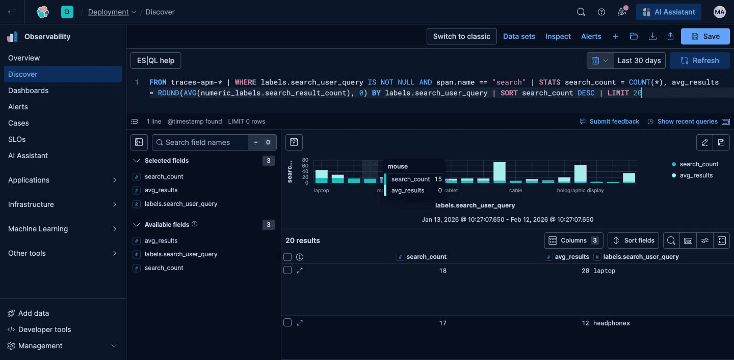
Set the time range wide enough to capture your data (top-right date picker). If you're just getting started, try "Last 30 days".
Six ES|QL queries for search analytics
Everything below runs against traces-generic.otel-default, the index where Elastic's OTel-native ingestion automatically stores trace data. You don't need to create this index; it's provisioned by Elastic when the first OTLP span arrives.
These queries ran against our live demo cluster: 62 searches, ~20 distinct queries, latency range 77ms–153ms.
Note: Results below are illustrative. When you run the reference project and generate traffic with python generate_traffic.py --blog 2 --sessions 50, your exact numbers and top queries will vary based on session count and random query selection. The query patterns and ES|QL syntax are what matter here.
Query 1: Are spans arriving?
Start simple. Count your search spans.
Result: 62.
If this returns zero, your spans aren't arriving. Check your OTLP endpoint and API key and that init_otel() is being called before any requests. The name == "search" filter ensures that you're counting your custom spans, not the auto-instrumented Elasticsearch client spans (which are also named "search").
Query 2: What are users searching for?
The first question every search team asks.
Results:
| Query | Searches | Average results |
|---|---|---|
| laptop | 9 | 8 |
| headphones | 7 | 12 |
| running shoes | 6 | 5 |
"laptop" was the most popular query, with nine searches. There were around 20 distinct queries total (including zero-result ones).
The avg_results column tells you whether popular queries are actually returning content. A query with high volume and low results is a relevance problem worth investigating. If your query has high volume and high results, check whether users are actually clicking. We'll get to that in the next blog focussing on measuring search quality with click data.
Query 3: What percentage of searches return nothing?
Result: 17.7% (11 out of 62 searches returned nothing).
We're using attributes.search.result_count == 0, a straightforward numeric comparison. No separate boolean attribute is needed when you already have the count.
A zero-results rate above 10% is worth investigating. Every zero-result search is a user who asked for something and got nothing back. Some of those are junk queries, but others reveal real content gaps or query parsing failures.
Query 4: Which queries return nothing?
The rate tells you there's a problem. This query tells you where.
Results:
| Query | Occurrences |
|---|---|
| quantum physics calculator | 4 |
| unicorn saddle | 3 |
| holographic projector | 2 |
| time machine parts | 2 |
Three different failure modes: "quantum physics calculator" and "unicorn saddle" are out-of-catalog queries you'll never be able to serve. This is useful to know but nothing to fix. "holographic projector" might be a real emerging category worth considering. "time machine parts" is probably noise. In a production catalog, these would be mixed with legitimate zero-result queries that are fixable, like missing synonyms, phrasing mismatches, or product gaps.
Repeated zero-result queries are the highest-priority fixes. One-off failures are usually noise.
Query 5: How fast is search?
Result: Average 81ms, max 153ms.
search.took_ms captures Elasticsearch's self-reported execution time, the took field from the search response. This is different from span duration, the wall-clock time from when the span started to when it ended (as we covered in the primer above). Span duration measures end-to-end time, including network round trips, serialization, and application logic. You want both: Comparing them tells you where overhead lives. If took_ms is 50ms but the span duration is 200ms, the extra 150ms is network or application overhead, not a query problem.
This attribute also keeps your analytics portable. If you're using OTel log records instead of spans (a lighter-weight alternative we mention in the first blog in the series), there's no span duration. took_ms is the only timing signal you have.
We'll go deeper on search performance monitoring (Service Level Objectives [SLOs], alerting on latency regressions, and using this data for operational dashboards) in the last blog in the series focussing on Search Reliability Engineering.
Want to find the slow queries specifically?
A query with high average latency and high result count is hitting many documents; consider query optimization. High latency with low results might mean complex filters or slow aggregations. Outlier max values are often cold caches or cluster issues.
Query 6: How does search volume change over time?
Counts, rates, and latencies tell you the what. Volume over time tells you the when: When did traffic spike, when did it drop, and when did that zero-results rate jump?
DATE_TRUNC(5 minutes, @timestamp) rounds each timestamp down to the nearest 5-minute boundary. The result is a time series that Kibana's Lens can render as a bar chart or line, showing your search traffic pattern for any time window.
Narrow the bucket for higher granularity (1 minute), widen it for trend analysis (1 hour, 1 day). When you add this to a dashboard alongside your zero-results rate, you can answer: Did zero-results spike because traffic changed or because something broke?
Verify that your search API instrumentation is working
If you're using the reference project, the full setup is:
Then trigger a search:
Wait 5–10 seconds for the BatchSpanProcessor to flush, and then open Kibana → Discover → switch to ES|QL mode and run:
You should see rows with attributes.search.query, attributes.search.result_count, and attributes.search.took_ms.
If no rows appear, check in order:
OTEL_EXPORTER_OTLP_ENDPOINTpoints to the mOTLP endpoint, not your Elasticsearch URL.OTEL_EXPORTER_OTLP_HEADERSincludesAuthorization=ApiKey <your-key>.OTEL_TRACES_SAMPLER=always_onis set (default sampler may drop spans).- Kibana → Observability → APM → Services shows
search-analytics-demo(confirms export is working).
Turn ES|QL results into Kibana visualizations
The bar chart that Discover auto-generates from your ES|QL results is a good start, but you can customize it. Click the pencil icon in the top-right corner of the chart to open the inline Lens editor.
From here you can:
- Change chart type (bar, line, area, pie, table, metric).
- Adjust axes and add breakdown dimensions.
- Save the visualization to a dashboard.
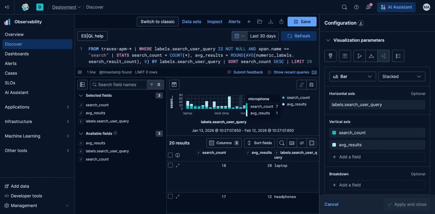
This is the path from ad hoc ES|QL exploration to a persistent dashboard panel. You don't need to build visualizations from scratch; Discover and Lens handle the chart rendering from your query results.
Lens is Elastic's drag-and-drop visualization editor, and it's more capable than this quick workflow suggests. You can build multilayer charts, combine metrics with breakdowns, add reference lines, and design full dashboards that mix ES|QL panels with traditional aggregation-based visualizations. For search analytics, that means you can put top queries, zero-results trends, and latency percentiles side by side in a single view.
To go deeper:
- Lens documentation: A full guide to the visualization editor.
- ES|QL in Lens: Using ES|QL queries as data sources for dashboard panels.
- Kibana Dashboards: Building and sharing operational dashboards.
- Use an Agent built in Kibana to make visualizations for you
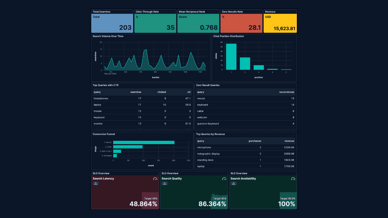
We'll build a full search analytics dashboard in a later post.
How sampling affects search analytics accuracy
Most application performance monitoring (APM) configurations sample traces to control costs, capturing 10% or 25% of requests. For application monitoring, that's fine. For search analytics, it's a problem.
If you're sampling at 10%, your "total searches" count is 90% lower than reality. Your zero-results rate is still accurate (it's a ratio), but volume counts are off.
Two approaches:
Approach 1: Configure 100% sampling for search endpoints. Your search API probably handles far fewer requests than your main application, so the data volume increase is manageable. The simplest way is through environment variables:
These are head-based sampling decisions made at the start of each trace. They apply globally to the service, which is fine if your search API is a dedicated service. If search shares a service with other endpoints and you need per-endpoint sampling rules, you can implement a custom Sampler in the OTel SDK that inspects the span name or attributes before deciding.
More sophisticated routing (sampling differently per endpoint, dropping noisy spans, or making decisions after a trace completes [tail-based sampling]) typically involves deploying an OTel Collector (such as the EDOT Collector) as an intermediary between your application and Elastic. That's a valuable architecture pattern, but it's beyond the scope of this post. See the OTel Collector documentation and Elastic's EDOT Deployment for more on collector-based sampling and routing architectures.
Approach 2: Upscale in your queries. If you know the sampling rate, multiply: EVAL estimated_total = total_searches * 10. Ratios and averages stay correct; only absolute counts need adjustment.
For more on sampling strategies generally, see the OTel sampling documentation.
For the queries in this post, we used 100% sampling.
What's next: Adding click tracking to search analytics
The six ES|QL queries in this post answer: What do users search for, what returns nothing, how fast is search, and when does traffic spike? They're all derived from a single instrumentation point: the search span.
But they can't tell you whether users are finding what they need. A search that returns 15 results looks healthy from the server side. But if nobody clicks any of those results, your ranking has a problem.
In the next post, we add click tracking, a second span that captures which result the user clicked and where it appeared in the list. If you've been running the reference project, you already have 62 search spans; the next post builds directly on that data. With searches and clicks linked together, we'll calculate:
- Click-through rate (CTR): What percentage of searches result in a click.
- Mean Reciprocal Rank (MRR): How far down the results users have to scroll.
- Click position distribution: The shape of where users click.
The pattern is the same: You add attributes to spans and query them with ES|QL. You get a richer view of the same data without introducing new infrastructure.
Resources to get started with search analytics on OpenTelemetry
- Reference project: Working code for the entire blog series; clone, configure, run.
- EDOT Python: Elastic distribution of OpenTelemetry for Python.
- OpenTelemetry with Elastic: How to send OTel data to Elastic APM.
- OpenTelemetry Python SDK: Upstream SDK documentation and instrumentation guides.
- ES|QL documentation: Query language reference.
- UBI Standard: Reference schema for search event structure.
This is the second post in a series on search analytics with OpenTelemetry and Elastic. Next up: Measuring search quality: Click tracking, CTR, MRR, and click position analysis.
Contenido relacionado

9 de julio de 2026
Why Elasticsearch is becoming a columnar database
Elasticsearch is becoming a first-class columnar database. Columnar Mode ships in 9.5, storing data once alongside the existing modes and cutting storage footprints while speeding up analytical queries.
How to build search analytics on Elastic using OpenTelemetry, no extra pipeline required
How to instrument your search application to use modern Open Telemetry standard to drive insights in to your search and users.
Follow the money: tracing laundering networks with ES|QL and cross-cluster search
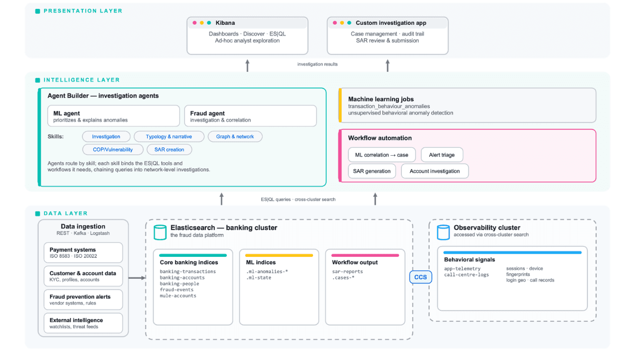
The data model, cross-cluster architecture and five ES|QL queries that power mule detection and laundering network tracing, built from infrastructure most financial institutions already run.

1 de julio de 2026
One command. Natural language. Your Elasticsearch data, straight to the terminal.
Query your Elasticsearch data from the terminal in plain English. The official Elastic GitHub Copilot CLI plugin generates and runs ES|QL queries against your cluster. No Kibana, no manual syntax.
30 de junio de 2026
Building a multilingual voice agent with Elastic Agent Builder & Sarvam AI
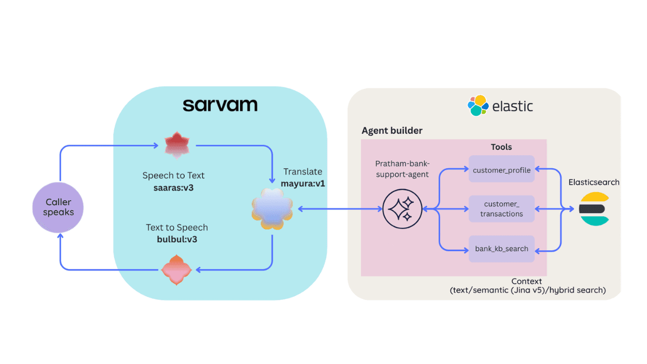
A working demo combining Sarvam AI speech with Elastic Agent Builder: identity verification, per-customer ES|QL queries, and mid-call language switching across 22 Indian languages without multilingual indices.