Get hands-on with Elasticsearch: Dive into our sample notebooks in the Elasticsearch Labs repo, start a free cloud trial, or try Elastic on your local machine now.
Elasticsearch now stores OTel metrics at 3.75 bytes per data point — down from 25 bytes a year ago — and queries them up to 30x faster and with up to 2.5x better storage efficiency, compared to Prometheus, Mimir and ClickHouse. These gains came from rebuilding TSDS storage and the ES|QL compute engine into a fully columnar metrics engine, with native OTel ingestion added as part of the effort — all while keeping Elasticsearch's ability to store and query logs, traces, and any other data alongside metrics.
Elasticsearch has supported storing metrics in time-series data streams (TSDS) since version 8.7. This offering mainly focused on storage gains as explained in an earlier blog post. Still, performance was not on par with specialized systems for storing and querying metrics, in terms of storage efficiency, indexing throughput and query latency.
In the past year, we revisited the storage layer, optimized ingestion for OTel metrics and extended the ES|QL compute engine with vectorized processing for time series data. These efforts led to substantial performance wins across the board, compared to earlier versions of TSDS:
- Up to 6.6x improvement in storage efficiency, reaching 3.75 bytes per data point in OTel metrics
- Up to 50% improvement in indexing throughput for OTel data
- Up to 160x improvement in query latency, including blazing fast counter rate evaluation and window support in time series aggregations
Elasticsearch has thus become a leading columnar metrics engine, matching or exceeding the competition (like Prometheus, Mimir, and ClickHouse) in indexing throughput and exceeding it by up to 2.5x in storage efficiency and 30x in query performance. All while maintaining the ability to store logs and other data and fully use the rich querying capabilities of ES|QL (e.g. inline stats, lookup join) — which other PromQL-based systems lack. Elasticsearch can thus serve as a unified storage and query engine for all user data, with no compromises for metrics and observability applications.
How TSDS is organized
TSDS has the following properties that help improve the performance of time-series codecs and produce correct results when aggregating data points per time series:
- The metric name and the dimension names and values are used to calculate the
_tsid, a unique identifier per time series. - TSDS get sorted by
[_tsid ascending, timestamp descending]order. Each time series is thus stored in sequence on disk, with newer data points appearing first. Since the_tsidis calculated over dimension values, the latter are also clustered on disk. - Shard routing is based on
_tsid, with each_tsidvalue appearing in one shard only. - Backing indices are time-bound, with no overlap over time between them.
The rest of this post explains how we use these properties to improve storage, indexing, and query performance.
Storage optimizations
TSDS already achieved a very competitive storage footprint, reaching 0.9 bytes per data point, when it is possible to combine many metrics in a single doc, sharing the same dimension values. However, when most data points have a unique set of dimensions (which is typical for OTel or Prometheus metrics), docs end up containing a single data point. In this setup, storage required 25 bytes per data point, with dedicated metrics stores requiring less than 10 bytes per data point.
To further reduce the storage footprint, we applied a series of optimizations over the past year:
Replace inverted indices and BKD trees with doc value skippers
Elasticsearch creates inverted indices (for text values) or BKD trees (for numeric values) by default for all non-metric fields, i.e. for @timestamp and dimensions. These indices improve performance for queries including filters on these fields, but have significant impact to storage — effectively doubling the footprint for each field. More so, they are also processed during segment merging, increasing the cpu, memory and storage overhead and slowing down the system — especially in high ingest throughput scenarios, as is often the case with metrics.
Lucene has been extended with doc value skippers, a form of hierarchical sparse indices that store the minimum and maximum value of blocks of documents. Range queries can check these min and max values and ignore blocks that don't fall into the requested range. Skippers work particularly well on sorted fields. Since TSDS are sorted by [_tsid, timestamp desc], dimension values get also clustered on disk. It's therefore possible to replace indices on @timestamp and dimension fields with doc value skippers that amplify the columnar layout — each field stored in its own files, with no duplicate tracking of each doc for indexing purposes.
Doc value skippers have negligible storage overhead — replacing indices with them led to a reduction of 10 bytes out of the initial 25 bytes per data point in OTel. Moreover, they work very well in practice when queries include filters on time ranges or dimension values (including prefixes and regex) — there was no noticeable regression in query performance in our benchmarks when they replaced separate indices. Doc value skippers are enabled for TSDS by default since version 9.3.
Enable synthetic IDs
The _id metadata field was another big contributor to the storage footprint. TSDS has already been extended to trim the doc values once they were no longer needed for replication, but the inverted index was kept around to efficiently support the id-based APIs (Get, Delete, Update).
The ID value for TSDS is synthesized by combining the _tsid and @timestamp values that uniquely identify each data point. Since these fields are configured with doc value skippers, it's possible to replace the inverted index on _id with (a) retrieval of the _tsid and @timestamp value from the _id value, and (b) checks for matches using doc value skippers respectively. Care has to be taken to avoid expensive checks for duplicate IDs during metric ingestion, with segment-level bloom-filters keeping the overhead at bay.
Supporting synthetic IDs in metrics is a first for Elasticsearch. It led to a reduction of 5 bytes out of the initial 25 bytes per data point for OTel metrics, with no loss of functionality. Synthetic IDs are enabled for TSDS by default in version 9.4. We plan to extend their uses in logs and other applications after further evaluation.
Trim sequence numbers
Sequence numbers are used as part of replication, but also to provide strong consistency semantics on doc modification operations through Optimistic Concurrency Control (OCC). While such semantics are applicable to certain scenarios, they don't fit in metrics where concurrent updates are very rare, with no practical need for guarding against concurrent operations on data points with matching ids. We therefore decided to disable the use of sequence numbers in all APIs, along with OCC support, for TSDS, in version 9.4. This leads to a substantial storage reduction of 4 bytes out of the initial 25 bytes per data point for OTel data, as there's no inverted index and sequence numbers get trimmed once no longer needed for replication. Update and delete by query operations are still supported, albeit with weaker consistency semantics.
If OCC is still deemed important for a particular metrics application, the old behavior can be restored by setting index.disable_sequence_numbers: false in the index template of the involved TSDS.
Use large numeric codec blocks
TSDS already uses an advanced codec, as explained in an earlier article. The codec works very well in most cases, but has poor performance in case of repeated sequences of keywords and numbers, leading to an inflated storage footprint for dimensions containing IP and MAC addresses. We identified that the existing logic for identifying repeated sequences requires larger codec blocks to work well, especially as the sequence length increases. After experimentation, the numeric block size was increased from 128 to 512 elements in version 9.3, leading to a reduction of 2 bytes out of the initial 25 bytes per data point for an OTel dataset containing IP and MAC addresses as dimensions. We're also working on a more configurable codec layout that will allow more flexibility with block sizes and other parameters, based on field type and cardinality.
Indexing throughput
Elasticsearch has support for bulk ingestion of documents. This entrypoint has long been optimized for leniency, ensuring that all docs get accepted. This flexibility, however, incurs additional processing cost during indexing. Metric applications proved good candidates for using different approaches to reduce this overhead, as explained below.
Introduce OTLP protobuf entrypoint
OTel metrics and Prometheus have established protocols for metrics ingestion, using protocol buffers. In the past, a translation step was required to convert collected protobuf messages to bulk requests that Elasticsearch can consume.
Elasticsearch was recently extended with endpoints accepting messages from OTel metrics collectors and over Prometheus remote write. Parsing and processing these (binary) messages is cheaper, compared to json parsing, while hash operation over dimensions for _tsid calculations get reused and amortized across more data points within a single protobuf message. Furthermore, _tsids get evaluated once per doc in the coordinator nodes and propagated to data nodes for indexing, thus deduplicating an expensive step per indexed doc. These improvements led to up to a 20% speedup in indexing throughput for OTel metrics. The OTLP entrypoint was added in version 9.2 (tech preview) and reached GA in version 9.3. We've added similar entrypoints for Prometheus remote write in version 9.4 (tech preview) and are actively working to cover OTel Logs and Traces.
Reduce indexing CPU with doc value skippers
In addition to a substantial storage footprint, inverted indices require a lot of cpu to build and reconstruct during segment merging. The use of doc value skippers in their place helps also reduce cpu load at ingestion and thus improves indexing throughput by 10%, a welcome bonus on top of the aforementioned storage wins.
Synthetic recovery source
The original source of a document, as provided at index time, is never stored for metrics. Still, Elasticsearch needed to temporarily store it for replication purposes. That changed in version 9.1, where the source gets synthesized on demand for replication purposes. This is known as synthetic recovery source and reduces disk I/O by 50%, with a significant impact to metrics indexing performance. Check out this article for more details.
Query execution
Replacing inverted indices with doc value skippers leads to a pure columnar storage layout for TSDS, with metric and dimension fields stored as Lucene doc values, each field encoded and compressed in their own file. Combined with the introduction of the ES|QL compute engine that uses vectorized execution internally, it became possible to introduce a fully columnar storage and query processing engine for metrics in Elasticsearch. We pushed this idea to the extreme and implemented a columnar metrics processing engine that comfortably outperforms dedicated metrics engines and other columnar stores in query performance.
Time series integration in compute engine
Time series processing is largely based on applying aggregation functions per time series (or _tsid), such as a gauge average or a counter rate. These partial results are then reduced by a secondary function to produce results for the grouping dimensions, e.g. per host and process. Observability dashboards are built on top of this execution model, providing summary views of how metrics evolve over time and allowing for quick deep-dives by filtering on dimension values and time ranges.
To support this execution model, we introduced the TS source command, providing a simple yet powerful syntax for executing such queries that combine an inner aggregation function per time series with an outer aggregation over the partial results of the former. For instance, the following query calculates the hourly sum of rate of search requests per host over the last day:
To execute this query, the compute engine is aware of how data is stored and applies the inner aggregation function per _tsid value. Since data are sorted by _tsid, time series aggregation functions process metric values as they get fetched, until the _tsid changes or the timestamp belongs to the next time bucket. This leads to vectorized execution of these functions over the fetched columns of metric values, while dimension values are only fetched (once) when the _tsid changes. The evaluation of the secondary aggregation function is also efficient, with partial aggregates stored in arrays of primitive values that get populated when _tsid values change.
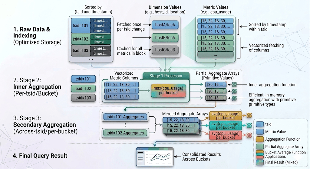
Vectorized time series aggregation execution
The compute engine has inherent support for parallel query evaluation, taking full advantage of the available processing cores. Time series aggregations fully use this feature and process data points in parallel as applicable, reducing response times through improved cpu utilization.
Time series processing in ES|QL was introduced in version 9.2 as tech preview and reaches GA in version 9.4. We expect all metrics applications to adopt it and benefit from the much improved query performance wins.
Zero-copy data decoding and loading
Vectorized processing of time series data delivered immediate performance wins (8x for some queries), compared to aggregations through the /_search API, but the performance was still inferior when compared to competitive metrics stores. Benchmarking and profiling showed that there were too many array copies within the compute engine, between data decoding and evaluation of aggregation functions. To that end, the following optimizations were introduced:
- The codec for TSDS was extended to decode on-disk data directly into primitive arrays inside blocks that the compute engine uses to evaluate time series aggregations. No additional copies required, as the compute engine can bulk-read these blocks and process their arrays, one column at a time.
- Blocks containing a single value N times are represented as constant blocks with these 2 values, as opposed to an array with length N, a form of in-memory run-length encoding. Filtering and aggregation operations were extended to efficiently consume these blocks. This reduced memory pressure and cpu overhead for the
_tsidand dimension fields, as their values get clustered due to index sorting. - Documents with null values for the aggregated metric fields are filtered out at the Lucene level, before they get decoded and copied into blocks.
- All filters and regular expressions on the timestamp and dimension fields get pushed down to Lucene that makes use of doc value skippers to efficiently filter out non-matching docs.
Combined, these optimizations led to query execution speedups exceeding 10x (totaling 80x when combined with the 8x speedup from vectorized execution). They were included since the introduction of the TS source command in version 9.2, and fine-tuned ever since.
Optimized counter rate evaluation
While most time series aggregations can be trivially parallelized and evaluated, rate evaluation of cumulative counters is tricky as it requires processing all data points in order to detect counter resets (e.g. when a host restarts). To address this, the compute engine uses the _tsid prefix to shard time series across threads. Care has been taken to assign in-order ranges of _tsid values to each thread, as opposed to hash-partitioning _tsids, so that each thread can scan on-disk data in order, still making use of efficient decoding and zero-copying into blocks. The performance wins are impressive, with rate evaluation performance far exceeding dedicated metrics stores as we shall see in the next section.
Another interesting problem for cumulative counters is how to properly calculate counter increases for the entire time bucket when there are no data points at the bucket boundary timestamps. Metrics systems often use extrapolation, extending the first and last data points of each time bucket to the boundaries, or calculate the delta between the last data point of adjacent buckets. We posit we can do better, by interpolating between the last data point of each bucket and the first of the next, to get an estimate of the value on each boundary. The delta is then calculated over the interpolated values of the lower and upper boundary of each time bucket.
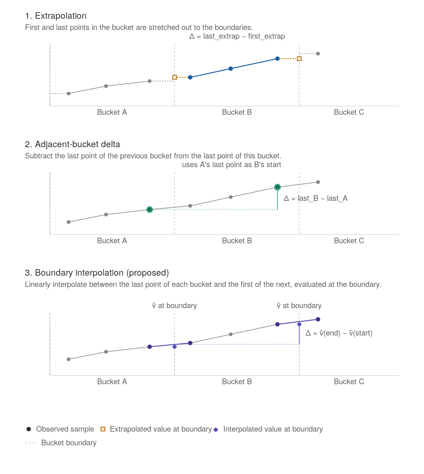
Counter rate interpolation across time bucket boundaries
Sliding window support
Elasticsearch has long supported aggregations bucketed by time, but it was not possible to extend the window of processed data beyond each time bucket. Using windows larger than the time bucket, e.g. a window of 5 minutes for per-minute bucketing, helps smoothen out spikes and observe the underlying trend per time series with reduced noise:
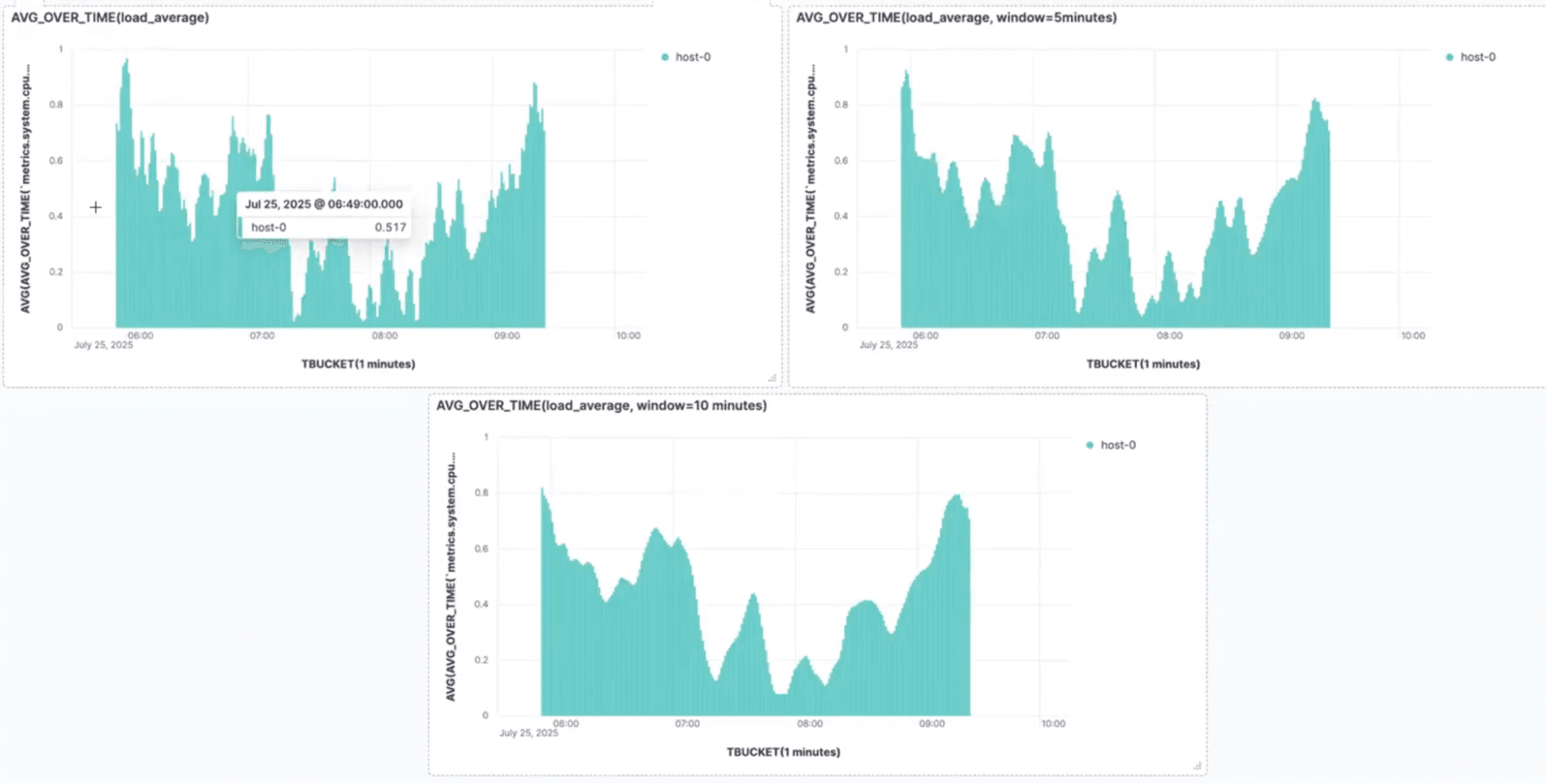
Sliding window smoothing example
All time-series aggregation functions have been extended with window support, as an optional argument. In case the window is a multiple of the time bucket (e.g. 1h window with TBUCKET(5m)), the compute engine first aggregates data points over intervals matching the time bucket span, and then combines these partial results per window span. This 2-phase approach eliminates repeated scans of data points and makes optimal reuse of intermediate results, improving response times. Window support was introduced as tech preview in version 9.3 and reaches GA in version 9.4.
Efficient datetime rounding
Queries on time-series data commonly include time bucketing. While data points can be trivially assigned to sub-hour time buckets, larger buckets start interfering with issues like time zones, daylight savings, variable days per month etc. Elasticsearch has elaborate logic for datetime rounding that takes these peculiarities into account, but that has relatively high cpu cost when processing time series data.
To mitigate this, the compute engine has been extended to identify cases where simpler logic can be employed to assign data points to time buckets. For instance, it can identify when the buckets are sub-hour or when timezones and daylight savings don't affect a particular query, and switches to simple modulo operations for datetime rounding. This led to a further 30% improvement in response times for certain queries. This change is introduced in version 9.4.
Performance evaluation
To evaluate the performance of our offering and track how it evolves and improves over time, we focused on OTel metrics since (a) Open Telemetry is the industry standard for collecting metrics, with universal adoption by all cloud providers and (b) they lead to a storage layout with 1 metric per doc, a setup that traditionally hurt performance for Elasticsearch.
We rely on Metricsgenreceiver to generate datasets. This tool is inspired by TSBS, producing data simulating the data points collected by the OTel hostmetricreceiver. We used two datasets:
- A low-cardinality setup, with 100 hosts sending metrics every 1s, containing 14k time series in total
- A high-cardinality setup, with 10k hosts sending metrics every 10s, containing 1.4M time series in total
We benchmarked on single-node deployments on EC2, using c6i.4xlarge and c8g.8xlarge machines for the low- and high-cardinality datasets respectively.
For competitive comparison, we used Prometheus (v.3.11.1), Mimir (v.3.0.6.) and ClickHouse (v26.3.9.8-lts). Prometheus and Mimir have proper time series processing, e.g. for counter rate, whereas ClickHouse lacks such support and only provides approximate values at best (for instance, it can't track counter resets consistently). We still report response times for ClickHouse to showcase that, once we optimize Elasticsearch for columnar query processing, it can exceed competing columnar engines even when they don't process the data per time series as expected.
We strived to use the default configuration for every system (including Elasticsearch), without tweaking them to optimize performance for the particular workload. This helps understand the user experience when systems are deployed by novice users, without much experience (or time) to tweak before receiving metrics traffic and setting up dashboards. We focused on single-node runs to keep noise low and accommodate all systems (Prometheus doesn't offer a multi-node setup out of the box). Elasticsearch performance provably scales well with the number of nodes; we plan to share scalability results in a future post.
Storage efficiency and indexing throughput
Our efforts to improve storage efficiency paid big dividends. Performance on OTel metrics dropped from 25 to 3.75 bytes per data point, in a year. Such an improvement, on top of an offering already optimized for time series, is really impressive and very rare in the industry.
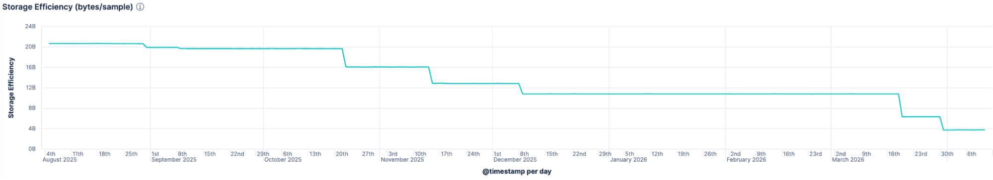
Storage efficiency improvements over time
The competitive picture looks favorable at this point, with Elasticsearch:
- Slightly outperforming Mimir in storage efficiency and indexing throughput
- Outperforming Prometheus by 2.5x in storage efficiency and by a small margin in indexing throughput
- Outperforming ClickHouse by 2x in storage efficiency and by 40% in indexing throughput
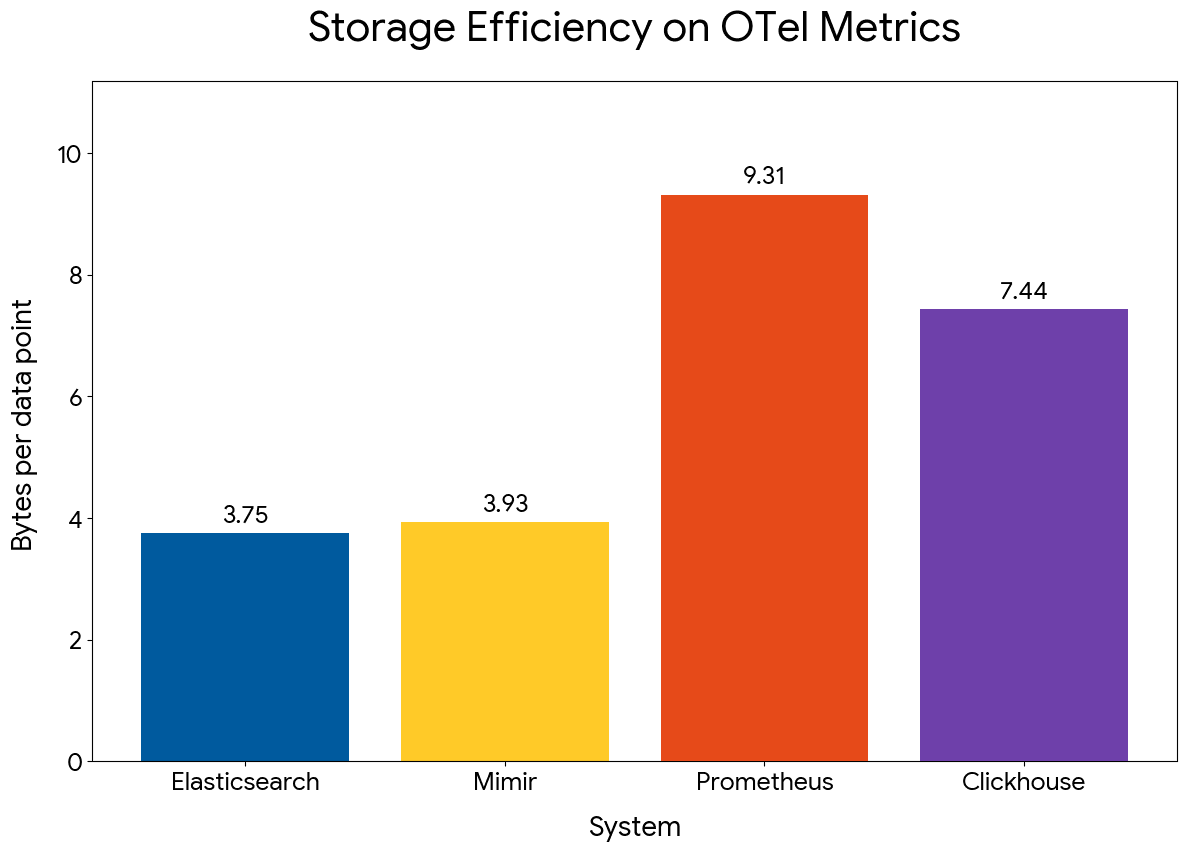
Storage efficiency comparison across systems
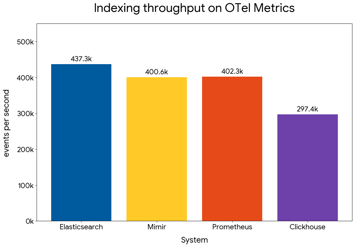
Indexing throughput comparison across systems
Query performance
The novel columnar engine for metrics processing proves very efficient in practice. We used a mix of queries based on gauge averages and counter rates, the most common operations that require different optimization approaches. The queried interval was 4 hours of data, covering all time series per metric.
ClickHouse doesn't support time series aggregations, so the results have limited value and are not directly comparable to Prometheus or Mimir that natively support time series processing. We used the published guidelines to adjust each query to get similar results to the extent possible. The point is to show how our columnar engine compares to generic columnar stores.
Here is a summary of the results:
| Query type | Mimir | Prometheus | ClickHouse † |
|---|---|---|---|
| Gauge average | up to 30x faster | up to 30x faster | up to 8x faster |
| Counter rate | up to 30x faster | up to 30x faster | up to 3.5x faster |
| Prefix filter on host name | up to 5x faster | up to 5x faster | up to 3x faster |
| Gauge average with window | up to 25x faster | up to 25x faster | up to 4x faster |
†ClickHouse lacks native support for time series aggregations and counter reset detection.
Gauge average
We compared performance of evaluating the per-host hourly average of average memory utilization per time series, using the following queries:
Elasticsearch comfortably outperforms the other systems by up to 30x, in both low and high cardinality datasets.
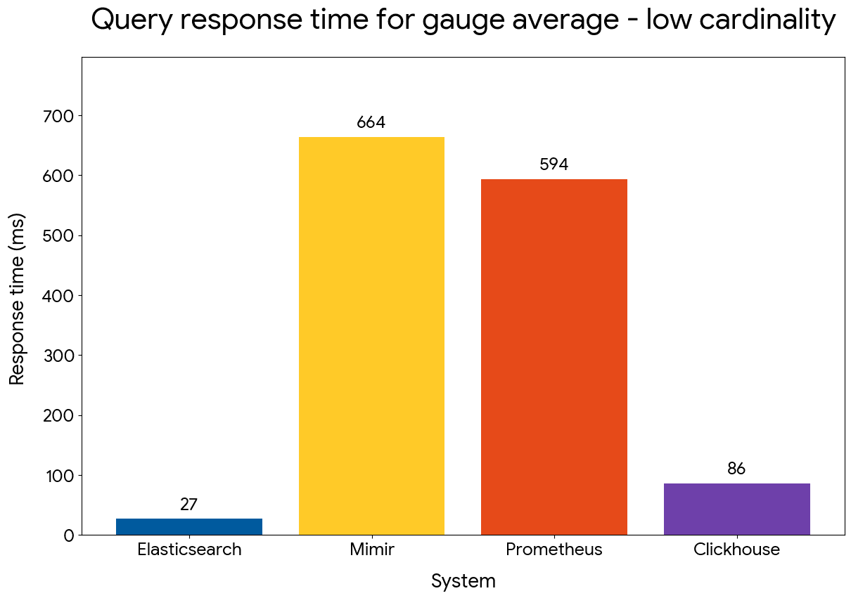
Gauge average query performance — low cardinality
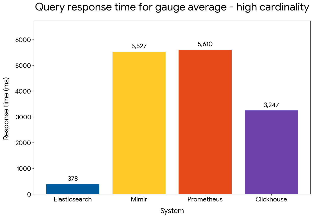
Gauge average query performance — high cardinality
Counter rate
We next compared performance of evaluating the per-host hourly average of cpu rate, using the following queries:
Despite processing data points per time series in order, counter rate performance matches calculating gauge average (the involved time series have 6.6x more docs than the query above). Elasticsearch maintains its wide advantage compared to the other systems and outperforms Mimir and Prometheus by 30x in the low cardinality dataset and by 16x in the high cardinality one.
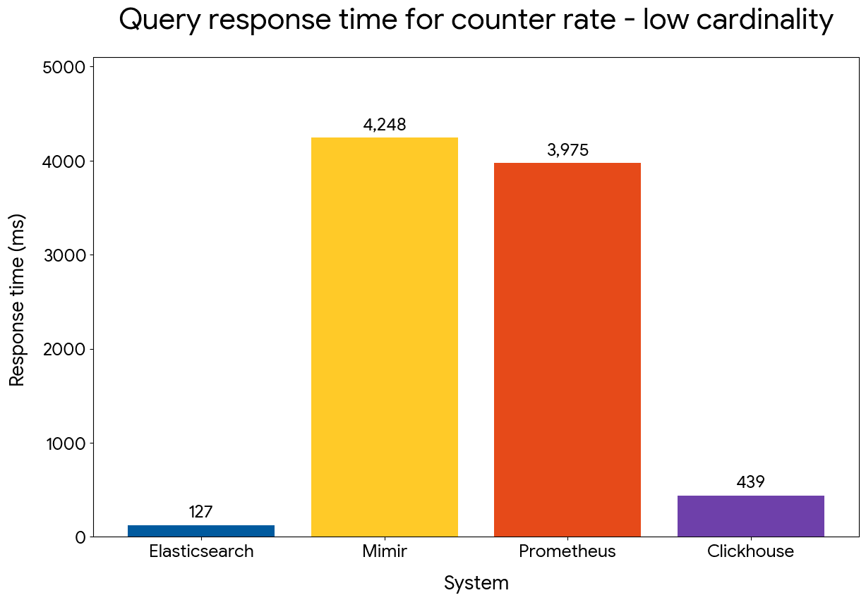
Counter rate query performance — low cardinality
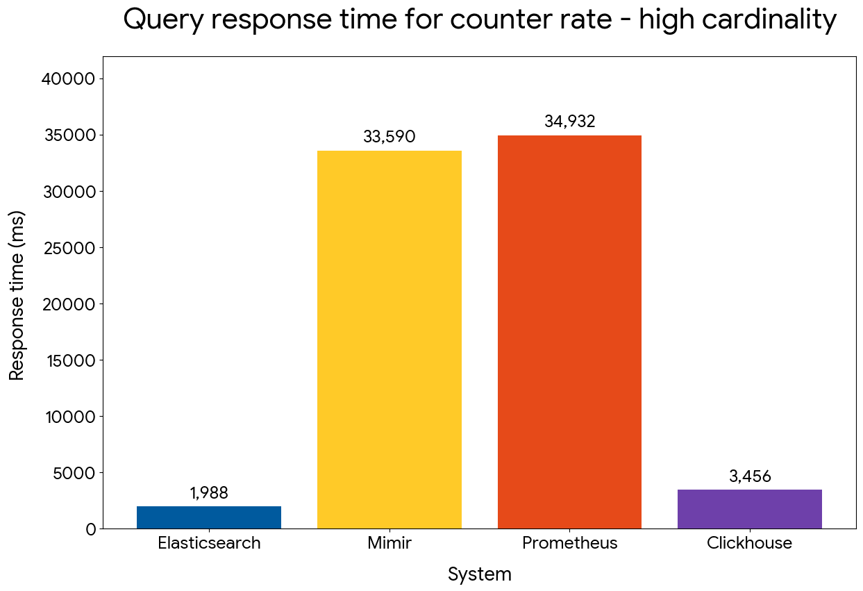
Counter rate query performance — high cardinality
It's really impressive that, for the high cardinality dataset, Elasticsearch is able to process 4 hours of data for half a million time series in less than 2 seconds, while the other systems take more than 30 seconds, leading to unresponsive dashboards for such queries. ClickHouse is also slower, despite having no logic to detect counter resets and extrapolate/interpolate deltas across buckets.
Prefix filter on host name
We next compared performance of filtering on host names based on their prefix, using the following queries:
Elasticsearch manages to maintain an advantage of up to 5x compared to the other systems, despite replacing the inverted index on host.name with a doc value skipper.
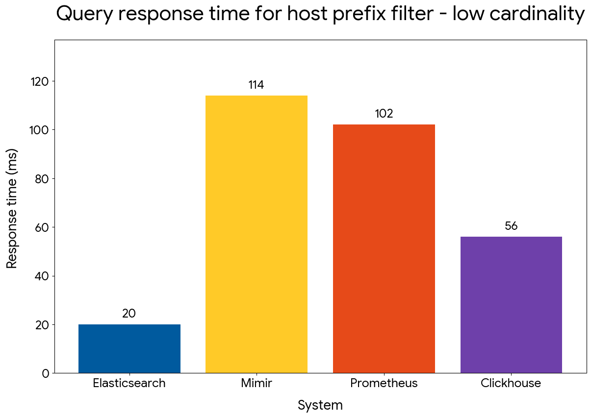
Prefix filter query performance — low cardinality
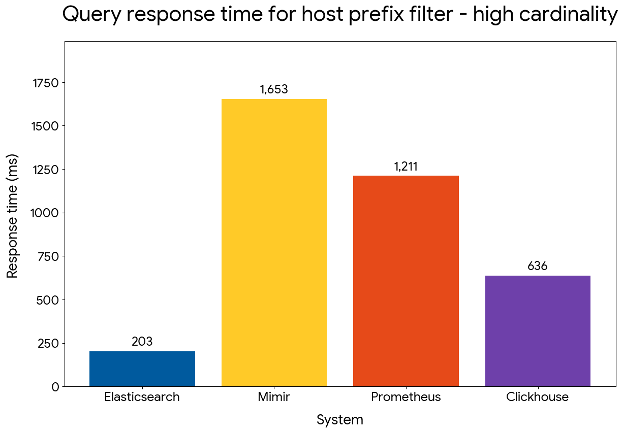
Prefix filter query performance — high cardinality
Gauge average with window
We compared the performance of time series aggregations with a window of 90 minutes and time buckets of 30 minutes, using the following queries:
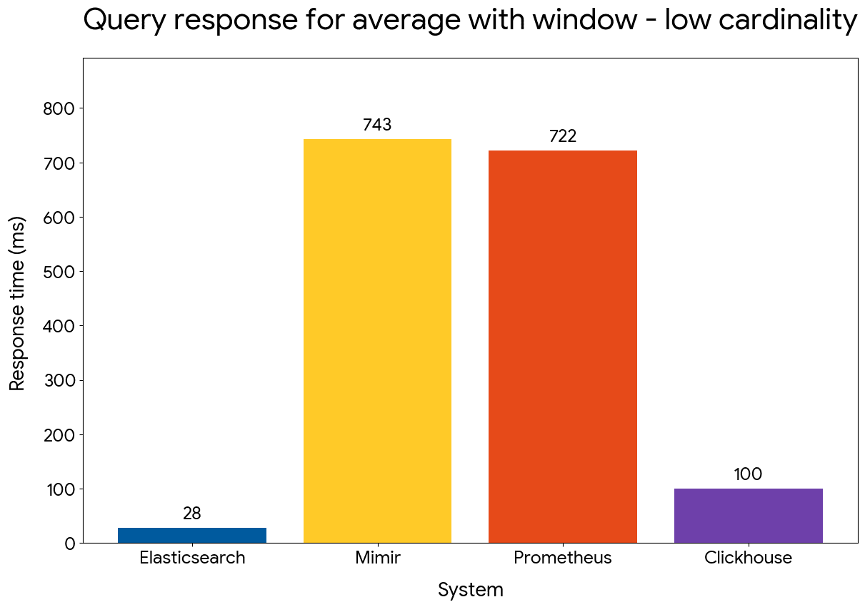
Gauge average with window — low cardinality
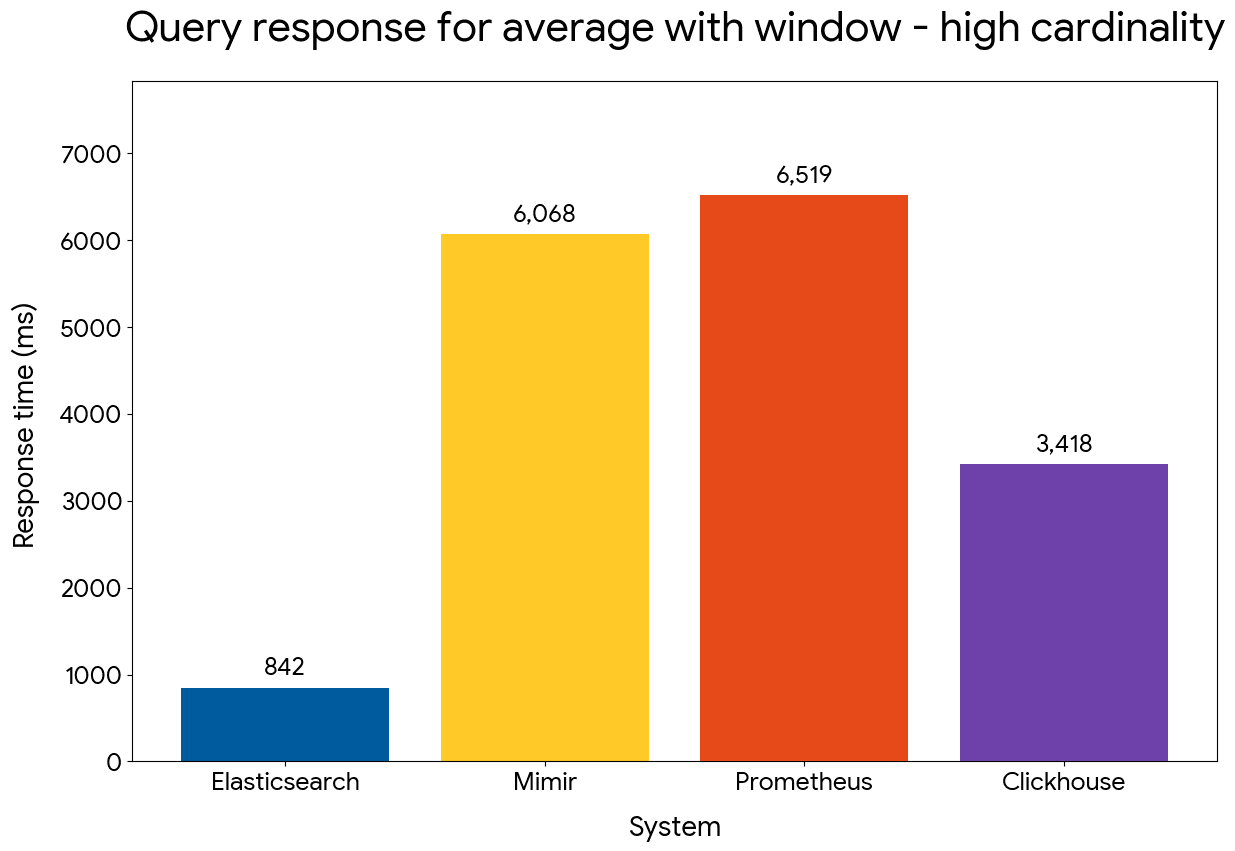
Gauge average with window — high cardinality
Elasticsearch maintains an advantage that reaches 25x for the low cardinality dataset and 8x for the high cardinality one. ClickHouse is outperformed by close to 4x, denoting the efficiency of our approach for windowed query operations.
What's next for Elasticsearch metrics
Elasticsearch has been extended with metrics storage and processing capabilities that outperform Prometheus, Mimir, and ClickHouse. We're making fast progress with supporting PromQL and Prometheus remote write, also available as tech preview in version 9.4. These extensions enable users familiar with Prometheus and relevant systems to switch their applications to Elasticsearch — no need to migrate existing dashboards. Since Prometheus integration reuses the same storage and query engine that has been presented in this article, the same performance wins are also expected for Prometheus. Furthermore, collected metrics can be queried with PromQL and ES|QL, side-by-side or in ES|QL query pipelines, further boosting the analytics capabilities far beyond what was conceivable so far with Prometheus-based systems.
The improvements in storage efficiency, indexing throughput and query performance are already impressive, but we're not done. We'll be introducing more refinements to the codec for time series data, further reducing bytes per data point. Batch processing of ingested metrics will be further improved, reducing synchronization overhead and redundant processing layers that are not needed for well-formatted collected metrics. We're also planning to make wider use of doc value skippers, storing pre-computed aggregates like sum and count per block of values, to shortcut data point loading and processing where applicable, as well as use more cpu-friendly partitioning and grouping operations.
Preguntas frecuentes
What is a columnar metrics engine and why does it matter?
A columnar metrics engine stores each field in its own file rather than row-by-row, then processes queries by reading only the columns needed. For time series data, this means Elasticsearch can decode metric values, dimension fields, and timestamps independently, applying vectorized operations across each column. The result is faster aggregations and lower storage overhead compared to row-oriented stores.
How does Elasticsearch compare to Prometheus for time series metrics storage and querying?
Elasticsearch stores OTel metrics at 3.75 bytes per data point in version 9.4, roughly 2.5x less than Prometheus. For queries, Elasticsearch outperforms Prometheus and Mimir by up to 30x in gauge average and counter rate benchmarks. For the high-cardinality dataset (1.4M time series), Elasticsearch processes 4 hours of data in under 2 seconds while Prometheus takes over 30 seconds.
What is Elasticsearch TSDS and when should I use it?
TSDS (time-series data streams) is Elasticsearch's storage format for metrics and time series data. It sorts documents by time series identifier (`_tsid`) and timestamp, stores fields in columnar doc values, and uses specialized codecs for compression. Use TSDS for any metrics workload, particularly OpenTelemetry or Prometheus data, where storage efficiency and query speed matter.
What is the TS source command in ES|QL?
`TS` is an ES|QL source command, GA in version 9.4, that executes time series queries using a two-level model: an inner aggregation per time series (such as `RATE()` or `AVG_OVER_TIME()`), then an outer aggregation over the results. The compute engine processes data in time series sort order, enabling vectorized and parallel execution. Example: `TS metrics | STATS AVG(RATE(cpu.time)) BY host.name, TBUCKET(1h)`.
How did Elasticsearch go from 25 bytes to 3.75 bytes per OTel data point?
Four storage changes contributed across versions 9.1 through 9.4: replacing inverted indices with doc value skippers (-10 bytes), enabling synthetic IDs (-5 bytes), trimming sequence numbers (-4 bytes), and increasing codec block size from 128 to 512 elements (-2 bytes). The result is a 6.7x reduction in storage footprint in roughly one year.
Can Elasticsearch replace Prometheus without migrating dashboards?
Elasticsearch supports Prometheus remote write (tech preview, version 9.4) and PromQL queries (tech preview, version 9.4). Existing Grafana dashboards using PromQL can point to Elasticsearch with minor modifications, and we expect to offer a seamless migration experience when our Prometheus offering reaches GA. The same TSDS storage and ES|QL compute engine power both PromQL and ES|QL queries, so the performance improvements apply to both.
What are doc value skippers and why do they matter for metrics?
Doc value skippers are Lucene index structures that store min/max values for blocks of documents. For TSDS, which sorts by `_tsid` and timestamp, they replace inverted indices on dimension fields and `@timestamp`. This reduces storage by up to 10 bytes per data point and cuts indexing CPU by about 10%, with no measured regression in query performance for time range and dimension filters.
Contenido relacionado
How to instrument your search API with OpenTelemetry and query it with ES|QL
Add custom attributes to OpenTelemetry spans and run six ES|QL queries that reveal your top searches, zero-result rate and slowest queries.

9 de julio de 2026
Why Elasticsearch is becoming a columnar database
Elasticsearch is becoming a first-class columnar database. Columnar Mode ships in 9.5, storing data once alongside the existing modes and cutting storage footprints while speeding up analytical queries.
How to build search analytics on Elastic using OpenTelemetry, no extra pipeline required
How to instrument your search application to use modern Open Telemetry standard to drive insights in to your search and users.

7 de julio de 2026
Your compliance posture just got an upgrade: Elasticsearch now supports FIPS 140-3
Elastic 9.4 brings FIPS 140-3 support for Elasticsearch and Kibana to GA. Here's what changes for federal, defense and regulated deployments, and how to migrate from 140-2.

2 de julio de 2026
A simdvec deep-dive: How Elasticsearch uses neural-net and video-codec CPU instructions for vector search
Four ways Elasticsearch's vector search engine reuses neural-network, video-codec and cryptography CPU instructions for up to 6x speedups; with the math, the failed attempts and the benchmarks.