Get hands-on with Elasticsearch: Dive into our sample notebooks in the Elasticsearch Labs repo, start a free cloud trial, or try Elastic on your local machine now.
As we discussed in our previous blog, we’re introducing fast approximate ES|QL STATS queries, which will be available in version 9.4 of Elasticsearch and the Elastic Stack. This feature allows users to estimate an expensive analytics query, often orders of magnitude faster than running the full query, by relaxing the constraint that it returns the exact value. We believe this has many uses; for example, we’re planning to integrate it into Kibana to obtain fast chart previews where possible.
In order for you to be able to trust our estimates, we provide error estimates. Furthermore, since there are edge cases in error estimation, we certify when the estimated value and error are trustworthy. In this blog post, we’ll dive into the theory for approximating and estimating the error in such queries, as well as discuss the testing we’ve done.
Background
In order to estimate ES|QL STATS queries efficiently, we make use of a property that’s shared by many statistics: Their estimates computed from a large number of independent samples from a dataset approach their true value. In the case of an index with some field we can think of the true value of a statistic as its value computed for a random variable with uniform discrete distribution on . In the following we denote this quantity ; it can be things like AVG, MEDIAN, and so on. If we make independent draws from , denoted , such that each value is selected with probability , we have independent copies of this random variable. The property we rely on means that a sample statistic value computed from approaches as becomes large. For example, if is the mean of some metric values then as becomes large. Indeed, for many statistics the limiting error distribution is known to be normal. Furthermore, it only depends on the distribution of , the size of the sample and the type of the aggregation . This means supported STATS queries can be approximated with fixed accuracy independent of the index size .
It is easy to pick values at random from a Lucene index: create a filter that takes exponentially distributed jumps through the dataset, where the expected jump size is controlled by the desired sample probability. The AND of this filter and any other Lucene query can be performed extremely efficiently, since AND’ing filter queries is one of the things for which it is well optimized. In our other post, we discussed some real-world query examples to give a sense of the speedup we obtain for different levels of accuracy.
So far, we've only discussed obtaining an estimate of a query. While such a point estimator can be useful, without knowing anything about its error those uses are limited. We found that ES|QL has existing capabilities that make it relatively easy to incorporate cheap, flexible, and accurate error estimation at the same time. We'll discuss this next.
Error estimates
We view providing an accurate understanding of the uncertainty in our estimates as crucial for users to be able to trust the approximation. While having the option to quickly estimate an ES|QL query alone can be useful in certain situations, we wanted to provide a richer feature that allows clients to make intelligent choices. For example, if an approximate query is being used to preview a chart and the error is only a couple of pixels, there’s little point in running another expensive query to redraw it.
The way we've chosen to represent error is by a confidence interval: the -central confidence interval, to be precise. This can be expressed in terms of the cumulative density, , of the statistic being estimated. Specifically, it's the interval which contains the true value of the statistic with probability whose endpoints are and . Confidence interval calculations are surprisingly subtle. There are also important constraints for our use case that make standard approaches undesirable. Next, we’ll take a look in more detail at the motivation and the design for the approach we’ve adopted.
A key requirement of the whole project is to dramatically accelerate expensive analytics queries. It’s therefore vital that the overhead of estimating uncertainty isn’t too large compared to estimating the query result itself. We also want the feature to be as general as possible, but “isolated” within the language. In other words, ES|QL is a flexible language, and we want estimation to work with as much of it as possible. At the same time, we don’t want to introduce a cross-cutting feature that incurs development costs on every new feature we ship.
With these considerations in mind, we chose to estimate confidence intervals by partitioning the sample set and computing the query output on each subsample. This is reminiscent of bootstrap; however, since we ensure that each partition receives a disjoint random subset of the sample data, we know that they comprise true estimates of the statistic distribution. To achieve the best possible estimate of the statistic itself, we still compute its value on the full sample. For example, to estimate the mean and its distribution the process can be expressed as follows:
This introduces a complication to account for the discrepancy between the count of values used to estimate a query statistic and used to sample its distribution. This is a downside; however, there are some significant advantages.
Most of the work in analytic queries resides in computing the aggregate statistics: post-processing after a STATS reduction acts on a far smaller table, and the cost is often relatively small. In this scheme, every row in the input data to the STATS command is processed exactly twice compared to just estimating the statistic. Therefore, roughly speaking we pay a fixed overhead that's the same order of magnitude as the cost of estimating the query in order to estimate its uncertainty. Since we often achieve multiple orders of magnitude speedup on the exact query, this is acceptable.
Because this process uses a plain old table, with extra columns for the distribution samples, we can pass the whole table through any ES|QL pipeline and compute confidence intervals on the final results. For example, if we include EVAL square_avg = avg * avg in the pipeline above, we'd have exactly the same square_avg, square_avg_0, …, square_avg_B-1 extra values. At the end of the pipeline, we have samples from the distribution of the original statistics and all quantities that are computed using them. Therefore, we can apply our standard confidence interval machinery to reduce the table and convert samples into confidence intervals for derived quantities as well. This whole process is essentially transparent to the rest of the ES|QL language, and as we showed above, can be achieved by query rewriting.
The confidence interval calculation
We have independent samples of the statistic distribution . However, they're computed with fewer values than our estimate . We also have a relatively small number of distribution samples, to avoid the count discrepancy being too large, and so we don’t inflate the table too much. We therefore prefer a parametric approach for estimating confidence intervals.
The errors in the statistics for which we support estimation tend to normal distributions in the limit they're computed from many values. So a natural choice, the standard interval, is to estimate the mean and standard deviation from the samples and report the corresponding normal confidence intervals . Here, denotes the standard normal distribution function. For heavy-tailed data and statistical functions that are sensitive to outliers, such as STD_DEV, convergence to normality can be slow, resulting in poorly calibrated intervals.
Briefly, in order to assess the quality of the intervals, one can examine their calibration. Specifically, one computes a quantity called the coverage. For a central confidence interval, it should contain the true statistic value roughly times for trials. In fact, since we seek the central confidence interval, we can make the stronger statement that the true value should be above, or below, the confidence interval endpoints in roughly out trials. The empirical coverage is this fraction computed for a large number of trials. It allows us to compare alternative approaches by simulation. We return to this when we report our test results.
In order to obtain better confidence intervals, we tried a couple of different approaches: the Cornish-Fisher correction of quantiles and an adaptation of bias-corrected accelerated (BCa) confidence intervals. Simulation showed BCa provided more robust calibration across a range of confidences, so this is the approach we selected. The basic idea, which was introduced by Efron, is to assume that there exists a monotonic transformation of the underlying statistic which, when applied to a distribution sample normalizes its distribution:
Here, , and is the standard normal random variable. This is clearly a relaxation of the assumption that the statistic itself is normally distributed, which is used to derive the standard interval. In fact, this family includes many distributions, since is only constrained to be monotonic. (You can think of as a first-order Taylor expansion of the case that the variance is an arbitrary function of the true parameter value. This further relaxes the assumption that the normalizing transformation also stabilizes the variance.) The nice thing about this ansatz is that never needs to be explicitly computed, and there exist standard approaches for estimating the parameters and from the distribution samples.
To handle one simply arranges for the estimate to land at the median of transformed distribution. If we assume the cumulative distribution function in theta space is then , where is the estimated statistic value, and as before is the standard normal distribution function. Typically, is approximated by the empirical distribution function, computed indirectly by bootstrap. However, somewhat surprisingly, extensive simulation showed that we obtained better calibrated intervals using a normal approximation to our sample values, i.e. with and their empirical mean and standard deviation, respectively.
To complete the procedure, one can rearrange (1) to derive quantiles for as follows:
where is the standard normal z-score for quantile . Typically, one uses the inverse empirical cumulative density estimate of to convert quantiles back to a confidence interval. However, because we have a mismatch between the count of values used to compute distribution samples and the query estimate, we need to do some sort of scaling. Exploring options by simulation, we again found it best to use a normal approximation, , where is the number of distribution samples we use. This is just applying the usual scaling of variance by .
Efron showed that in the case is distributed as , i.e. that it depends only on the true value , then the acceleration can be estimated without any knowledge of . In particular, . By assumption, our statistics tend to normal distributions with mean . Since skew is translation and scale invariant, this gives that , i.e. one sixth of the skew of our distribution samples. One thing this glosses over is the dependence of skew, and therefore acceleration, on sample size. We know it tends to zero as the count increases. In fact, skew also asymptotes to zero as and so we also adjust acceleration to be to account for the count mismatch between the samples and estimate .
Although we significantly improve the calibration of confidence intervals by using a better methodology, we still see issues in the case that the underlying distribution has very heavy tails for some of the supported STATS functions. Therefore, we introduce some additional guard rails we discuss next.
Guard rails
To avoid the user having to understand too much about edge cases, we provide additional safeguards that surface when we've been unable to confirm that the distribution samples behave as we expect. This typically happens when the statistic isn’t computed from a sufficient number of values given the metric distribution. It's exacerbated by very skewed metric data and certain aggregation functions, such as the STD_DEV, which are sensitive to outliers.
We have some global constraints on the minimum count of values used to estimate a statistic for which we'll certify it. For example, if any bucket is empty, then we can’t rely on the distribution samples. This is because ES|QL allows mixing approximate statistics, which treat empty buckets differently. For example, consider the following query:
There is no self-contained way of correctly assigning a value to mix for empty buckets, since summing requires that we treat them as zero, in which case we bias our estimate of avg. Alternatively, ignoring empty buckets introduces bias in the sum. There is also a global minimum count of values for which we’ve verified our certification method is sufficiently reliable; this is 10.
We explored a variety of additional tests to certify the results. These were based on both tests of the underlying data distribution, specifically Hill’s estimator, as well as the statistic’s distribution properties. If the true distribution of the statistic is sufficiently normal, then our estimate and confidence interval calculation behaves as we expect: The interval is well calibrated and the interval width is representative of the actual error. Therefore, in the end, we chose to use a test based on the p-value for distribution samples’ skewness and kurtosis versus a normal distribution null hypothesis. To certify a result, we require that the two tail p-values are greater than 0.05 for both tests. As we show below, we found this test was well aligned to our actual needs: to distinguish results for which the estimate and its confidence interval are more and less reliable.
There's a simple trick we can use to boost the accuracy of the accuracy of the test: Create multiple independent distribution samples and use a vote. Given a test to certify results with a failure rate , the distribution of the count of failures for tests is for the case the null hypothesis, that the estimate is trustworthy, is true. For example, for the majority vote assuming and then the significance of the test is , i.e. we fail to certify fewer than 1% of trustworthy results. Note that we can compute multiple trials relatively easily using different seeds for the RANDOM bucket identifier.
This additional check allows us to certify that we trust our estimates and their errors. We surface this information in the approximate query results. When we can’t certify results, they won’t necessarily be inaccurate, but they should be treated with more caution.
Testing
The two main aims of the testing we discuss here were to understand the calibration of the confidence intervals and to see how well they characterize the statistics' estimation errors. The count function is particularly well behaved, its error distribution is binomial, so the majority of our testing focused on metric aggregations. We study smooth distributions but make sure we cover a range of tail behaviors. The presence of outliers is the key factor that reduces the accuracy of estimated statistics. For example, if an outlier isn’t sampled at all, it can significantly affect the value of some statistics.
We explored a range of light-tailed distributions, such as uniform and normal, and skewed and heavy-tailed distributions, such as exponential, log-normal, Cauchy, and Pareto. For each family of distribution, we used multiple parameterizations, focusing primarily on varying the scale parameter. In total, we had 24 distinct data distributions. Figure 1 shows some example sample distributions from this set. Note that we’ve truncated the charts to remove extreme outliers, which are present for both the Cauchy and log-normal distributions.
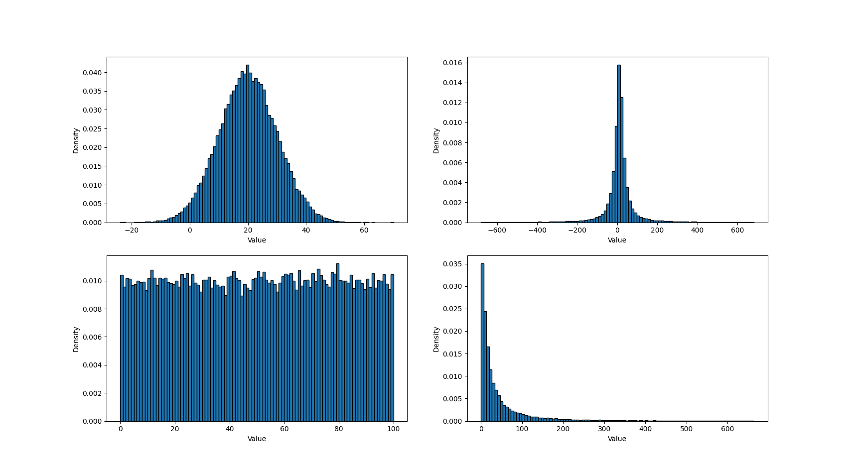
Figure 1 - Example metric sample distributions
For each data distribution, we evaluated 14 different sample sizes, ranging from 1000 to 500000. Then, for each sample set, we evaluated AVG, COUNT, MEDIAN_ABSOLUTE_DEVIATION, MEDIAN, PERCENTILE([25, 75, 90, 95, 99]), SUM and STD_DEV at two levels of confidence, 50% and 90%. In total, we have around 7500 distinct experiments. For each experiment, we assessed the interval calibration using 100 runs and counting the number of times the true statistic lands in the confidence interval. This gives us a binomially distributed estimate for the true confidence interval coverage. The variation we expect in the estimated coverage changes slightly with the level of confidence; for example, at 50% we expect to see values mainly between 0.44 and 0.56, and for 90% we expect to see values mainly between 0.86 and 0.94 using 100 trials.
Figure 2 shows box plots for the empirical coverage for the two confidence levels computed from all experiments. In all cases, the confidence intervals are reasonably well calibrated. Extreme percentiles are biased for small sample sizes, which leads to increased outlier counts for small sample sizes. As a rule of thumb, you’d want roughly samples to ensure that you have enough samples in the appropriate tail.
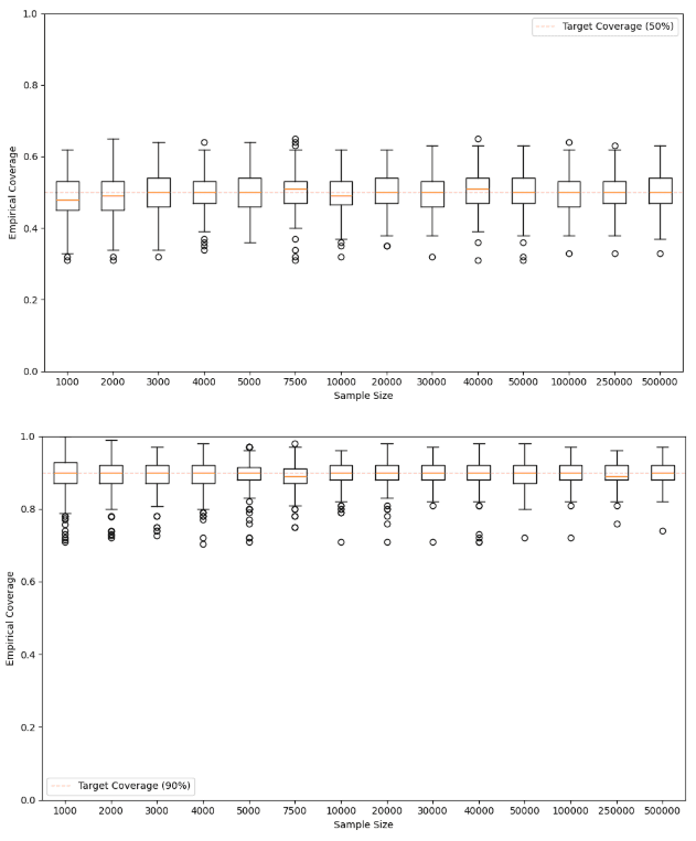
Figure 2 - Empirical coverage of the 50% and 90% confidence intervals for certified results
Next, we examine the degree to which the confidence intervals capture the typical size of the estimate error. To do this, we examine the distribution of the ratio of the estimated statistics' error and half the confidence interval width for all certified results. The higher the confidence, the wider the interval, so different confidence levels shift the mean of this distribution. Figure 3 shows this distribution computed for the 90% confidence interval. As expected, the distribution is roughly normal, albeit with a tail of some larger errors. We see in all cases the confidence interval width gives the order of magnitude of the estimated statistics' actual errors.
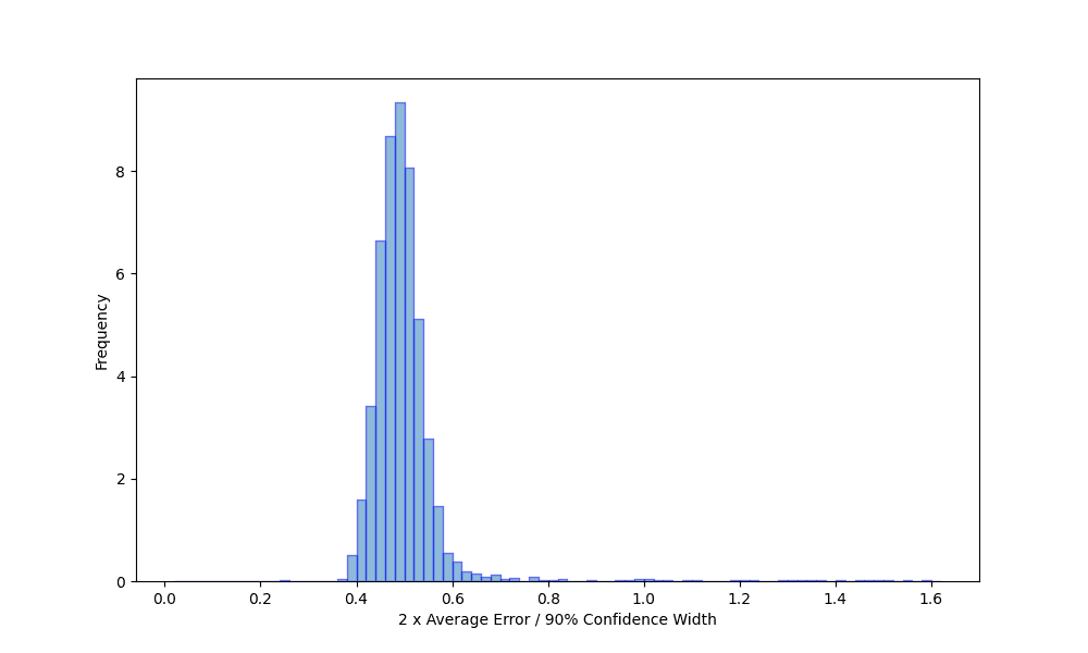
Figure 3 - Query error as a function of certified confidence interval width
We’ve shown that certified results are nearly always reliable; however, we’d also like some insight into the proportion of results which we fail to certify that are actually reliable, to confirm that the test aligns with our objective. We use reliable here in the fairly strong sense that the confidence interval is well calibrated. Specifically, for the 50% and 90% confidence intervals, we count the proportion of uncertified results for which the confidence interval empirical calibration has an acceptable margin of error, given the number of trials used to estimate it. Using this procedure, the false positive rate across all experiments is around 1%. This agrees well with the failure rate we expect by chance, given our test parameters, and confirms the assumption underlying the test.
Finally, to better understand the difference between certified and uncertified results, Figure 4 shows the error distribution of the ratio of the estimated statistics' errors and half the 90% confidence interval for the reliable and unreliable results separately. Note that we truncated the range for uncertified intervals.
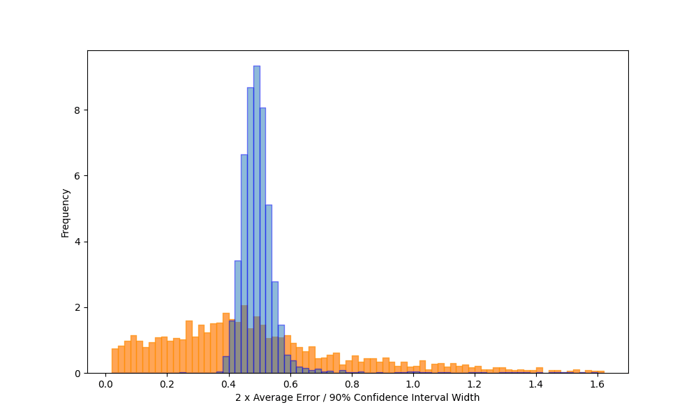
Figure 4 - Query error as a function of certified and uncertified confidence intervals
Wrapping up
In this post, we present the background behind our approach for quickly estimating ES|QL queries and providing an indication of their errors. To do this, we developed an effective confidence interval mechanism that allows us to provide error estimates. Our approach also allows us to estimate confidence intervals for quantities derived from sampled statistics via other pipeline operations. Quantifying the error comes with a relatively small overhead compared to just estimating the query. Finally, we developed a statistical test to certify results we return. Values that aren’t certified can still be accurate, but we’re less confident in them.
As well as testing the feature on a range of real-world use cases, which we discuss in our companion post, we tested the error estimation by extensive simulation across a range of data characteristics, sample sizes, aggregation functions, and confidence levels. This showed confidence intervals are well calibrated, and the interval itself provides a good approximation of the actual error we observe in the estimates. Finally, we showed that we were able to certify intervals with a low false negative rate.
We’re planning to integrate this feature into other stack capabilities in the future, so stay tuned.
Conteúdo relacionado

How to instrument your search API with OpenTelemetry and query it with ES|QL
Add custom attributes to OpenTelemetry spans and run six ES|QL queries that reveal your top searches, zero-result rate and slowest queries.

How to build search analytics on Elastic using OpenTelemetry, no extra pipeline required
How to instrument your search application to use modern Open Telemetry standard to drive insights in to your search and users.
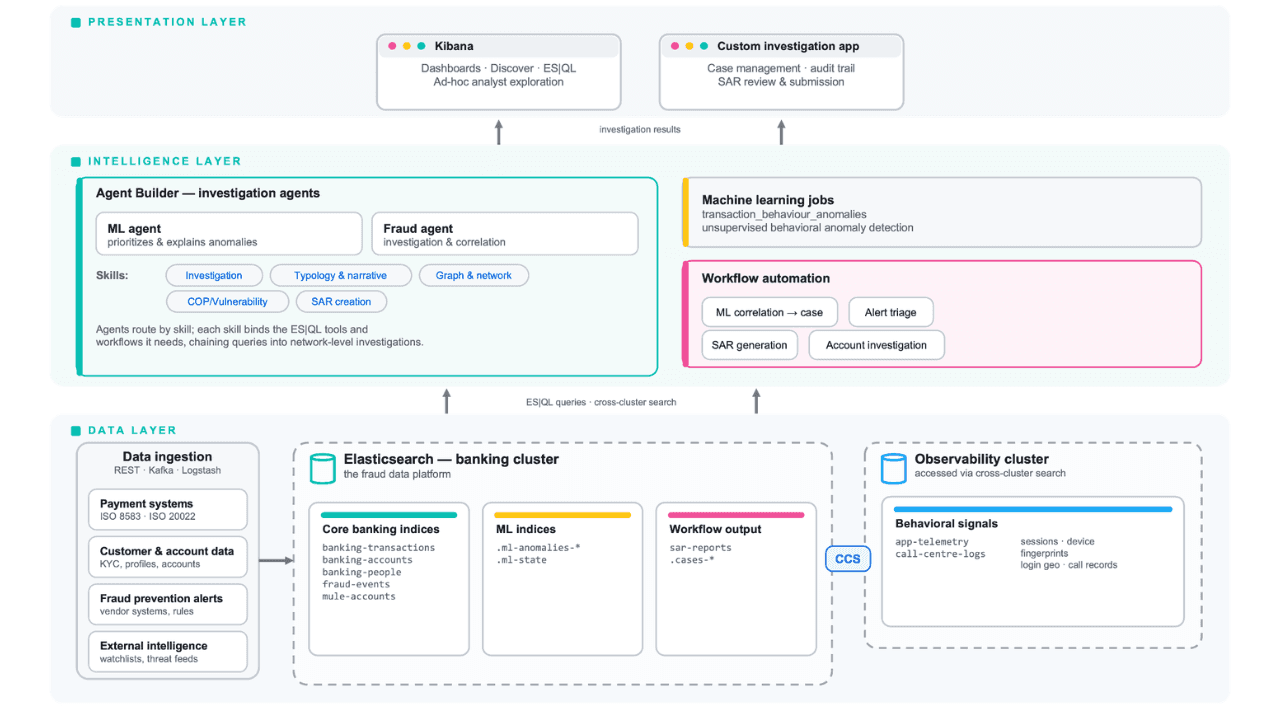
Follow the money: tracing laundering networks with ES|QL and cross-cluster search
The data model, cross-cluster architecture and five ES|QL queries that power mule detection and laundering network tracing, built from infrastructure most financial institutions already run.