Get hands-on with Elasticsearch: Dive into our sample notebooks in the Elasticsearch Labs repo, start a free cloud trial, or try Elastic on your local machine now.
Analytics workloads typically involve summarizing large volumes of data into a much smaller number of statistics. The Elasticsearch Query Language (ES|QL) implements this capability using the STATS command. This allows you to select various aggregation functions and apply them to the previous query results, as well as grouping the results by one or more ES|QL expressions. This is a flexible operation that, coupled with ES|QL querying capabilities, allows one to perform MapReduce on data stored in collections of Elasticsearch indices.
One of the key requirements for a pleasant user experience is that these operations are performed quickly. Large language model–based (LLM) agents also introduce new higher bandwidth and speculative query patterns that can potentially benefit from different optimization strategies.
In this two-part blog series, we discuss an optimization approach we’re introducing to ES|QL in version 9.4 of Elasticsearch and the Elastic Stack, which exploits a relaxation of the problem. Rather than trying to get exact values for aggregates, we allow ourselves to return approximate values, together with some characterization of their error. A key benefit of approximation is that it breaks the dependency between performance and dataset size: The accuracy with which one can approximate a query doesn’t depend on the original dataset size but, principally, its data characteristics and the query itself. As we’ll see later, this allows us to achieve some dramatic performance improvements.
In our next blog post, we will discuss the theory behind our approach and the validation we’ve done of its statistical properties. Here, we introduce the syntax and give a sense of how it’s achieved using standard ES|QL and query rewriting. You can explore its performance on a subset of the popular ClickBench benchmark. Finally, we discuss some limitations and gotchas that are worth understanding when you use query approximation.
Syntax and behavior
So how do you actually use it?
That’s it. You simply introduce the new line SET approximation=true; and write your STATS query pipeline as usual. Below, we discuss some advanced configuration options and some limitations around the agg(...) and commands. However, essentially, we choose defaults so that this will typically provide useful approximations while achieving significant speedups.
With this change, you’ll see some differences in the query results. Let’s look at a concrete example to illustrate this. Suppose the raw query is as follows:
The results might look something like this:
Approximating this query introduces some extra columns for each quantity that’s estimated:
The count column now contains an estimate, and you’ll see it’s somewhat different from the exact values above. The _approximation_confidence_interval(count) column defaults to the central 90% confidence interval for the count estimate and the _approximation_certified(count) column indicates if we’re highly confident that the results and their confidence interval are trustworthy. In outline, the confidence interval is an interval we expect has a high probability (0.9) of containing the true value for the quantity being estimated. The certified column indicates the distribution of the approximation is behaving as we expect. When the result isn’t certified, it’s often still accurate, but our test of the properties of its distribution hasn’t been able to confirm this. These quantities are discussed in more detail in our second post.
Implementation
An approximate query is rewritten before query execution using random sampling and extrapolation. Let’s take a look at the query of the previous section. The part of the rewritten query responsible for obtaining the best estimate looks like:
The query samples a fraction of the data, and therefore the final count has to be extrapolated by scaling up with the inverse of the sample probability. Extrapolation clearly depends on the underlying aggregation function, and we handle this appropriately for all functions we support.
To obtain the sample probability, we're setting a fixed number_of_rows to be processed by the STATS command. In this case, the probability is calculated as follows:
This query is executed before the final approximate query is executed.
As well as this best estimate, confidence intervals and a statistical test used to certify that the value distribution is behaving as we expect also need to be computed. The intervals are computed using a variant of the bias-corrected and accelerated bootstrap confidence interval (BCa) method. Therefore, the data needs to be partitioned into B buckets, which are used in turn to compute the intervals. Omitting some implementation details, this approximate query looks like:
To certify the estimate and confidence interval, there should be enough data, and the distribution of the bucket values should tend to normality.
Some queries can be efficiently computed using only summary statistics maintained in the index. To handle these correctly, where sampling is both slower and inaccurate, we updated the physical query planner, since detecting this case requires information that’s only available where the data resides. When the planner detects this is possible, it simply executes the query as normal. Such queries are typically fast anyway, and there’s no real side effect, so you don’t need to worry about this when using approximation; however, you’ll see that confidence intervals for such queries always have zero length, indicating the results are exact.
Results
To explore the performance improvements, we use ClickBench. This is a benchmark for analytics workloads for database management systems (DBMS). It comprises approximately 100 million rows, with a focus on clickstream and traffic analysis, web analytics, machine-generated data, structured logs, and events data. The benchmark also defines 43 queries that are typical of ad-hoc analytics and real-time dashboards.
Some of the queries aren’t suitable for approximation. For example, we don’t support approximating the unique count of a categorical value or computing the minimum and maximum of a metric value. We also don’t care about queries targeting search alone, for which Elasticsearch has excellent performance in any case. We therefore exclude these types of query from our evaluation. Finally, we also want to test a few additional aggregation functions, such as percentiles, which are not well represented in the original query set, so add some variants of the original metric queries to this end.
Queries in the benchmark are written using standard SQL and so need porting to use ES|QL syntax. This translation is fairly straightforward. Here’s an example:
becomes:
when rewritten in ES|QL.
For running all benchmarks, we use an Elastic Cloud Hosted instance with 870GB disk, 29GB Ram, and 4 vCPUs, in effect, an Amazon Elastic Compute Cloud (EC2) i3.xlarge instance. In the following results, we simply compare ES|QL with and without query approximation. Extensive results on a range of different hardware setups and datastores can be found here. Even with significantly constrained test hardware (matching the vCPUs of the smallest setup), our approximation approach achieves competitive results against much larger systems.
We run each query and its approximation five times in a random order, clearing the query cache between each run. We report the average run time over all five runs. While clearing the cache should be sufficient to avoid most of the advantage of running second, we wanted to avoid any possible accidental prewarming effects, which is why we alternate.
The results break down into four categories:
- Queries which are rewritten to use index summary statistics (three queries).
- Queries that perform well (13 queries).
- Queries with high cardinality partitioning (seven queries).
- Queries with restrictive filters (12 queries).
Roughly speaking, for these four categories, approximate querying is: equivalent (1); faster and accurate (2); faster but unreliable (3); and slightly slower (4), compared to exact querying, respectively.
For category 1, the planner automatically detects that we’re able to perform the query using summary statistics, and we end up executing the queries in the same way. To do this, we need information that’s only available on the data nodes, so we perform the rewrite only after we've estimated the sample probability. Because we're able to do this very efficiently, the overhead is small (around 10–15%). In both cases, the results are exact.
Queries in category 2 run on average 23 faster if estimating the values and computing confidence intervals and 72 faster if just estimating the values, which you can select as follows: SET approximation={"confidence_level":null}. These headline figures hide quite some variation in the impact of approximation on performance. The table below shows some queries sampled from the range of speedups we see:
| Query | Baseline / ms | Approximate with CI / ms | Approximate without CI / ms |
|---|---|---|---|
| 3 | 1725 | 145 | 15 |
| 10 | 4340 | 1721 | 56 |
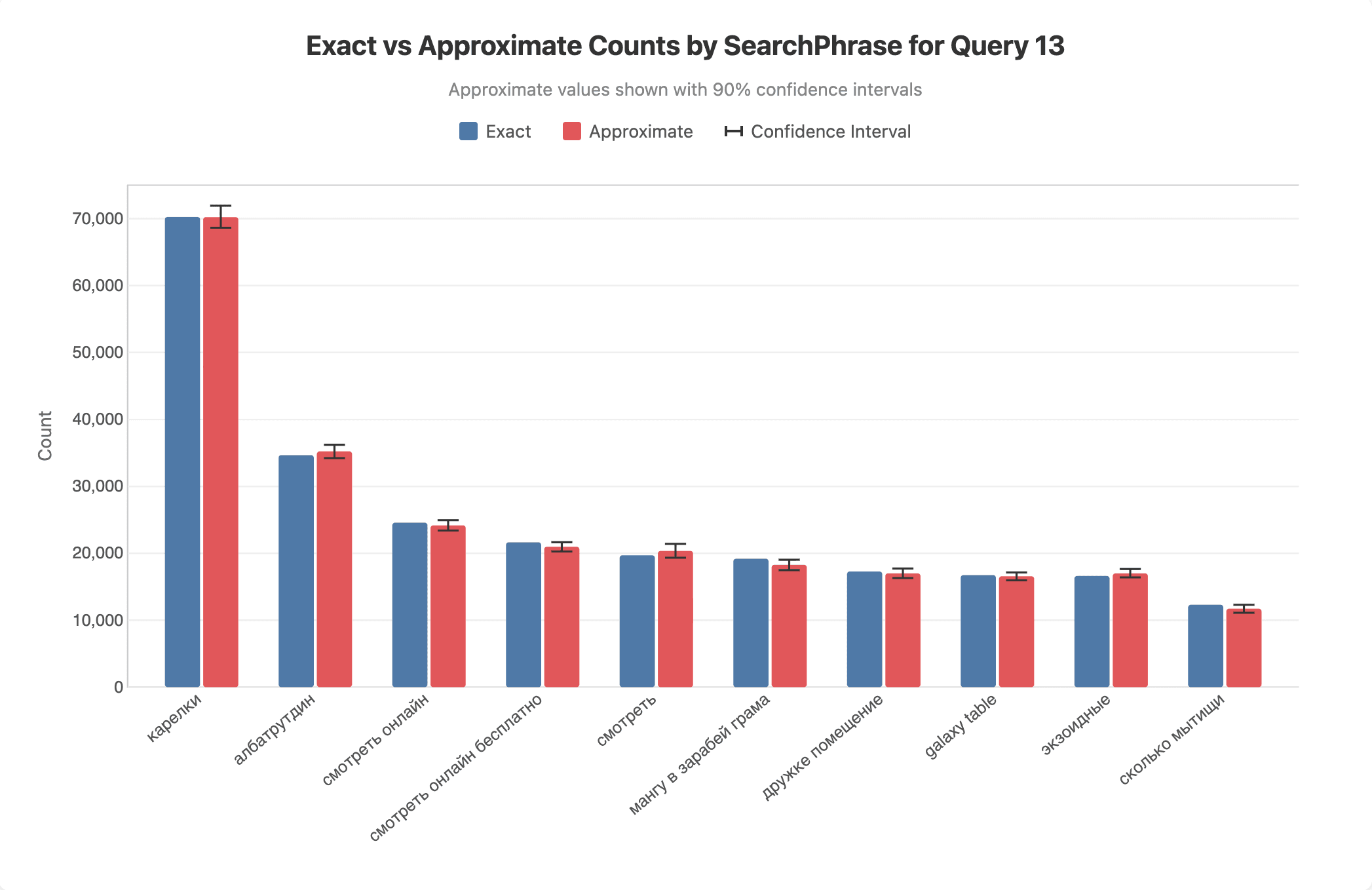
| 13 | 32912 | 6106 | 3821 |
| 21 | 46739 | 3284 | 2139 |
| 22 | 252505 | 6478 | 5019 |
Here are the corresponding queries:
We'll return to the accuracy of the approximation in the next blog post, but to give a sense of this, we plot below the exact and approximate values for a sample run for query 13:
For category 3, we get an average speedup of . However, the results of queries in this category can miss some partitions and often have large estimation errors. Approximation can still be valuable for such queries, particularly in the context of agentic workflows, but requires larger sample sizes than out default if accuracy is important. As we discuss in the next section, we provide an API to explicitly control the sample size. If the source dataset is sufficiently large, this can be increased and approximation will still yield significant performance improvements. The table below shows a couple of query examples for this category:
| Query | Baseline / ms | Approximate with CI / ms | Approximate without CI / ms |
|---|---|---|---|
| 15 | 8256 | 1187 | 124 |
| 17 | 70641 | 2109 | 982 |
Here are the corresponding queries:
Finally, category 4 queries use selective filters and end up being executed exactly, but they run slightly slower because of the work done in the query rewrite stage. Typically, all these queries run fast anyway, so the absolute slowdown is small. On average, they run approximately 14% or 370ms slower than the “without” sampling for our test setup.
Limitations and best practices
It’s worth explicitly mentioning some limitations. In particular, the following queries are not currently supported:
- Queries using the
TSsource command. - Queries using the
FORKorJOINprocessing command. - Pipelines which use two or more
STATScommands. - The
ABSENT,PRESENT,DISTINCT_COUNT,MIN,MAX,TOP,ST_CENTROID_AGGandST_EXTENT_AGGaggregation functions.
We plan to lift some of these restrictions in future releases, such as approximating queries using TS, FORK and JOIN; however, some are intrinsic. For example, while there’s prior art for estimating the minimum and maximum of a metric dataset or the count of unique values of a categorical dataset (see, for example, this paper), they require making certain distributional assumptions, either explicitly or implicitly. In summary, we view trying to automatically provide estimates of these statistics as being too open to accidental misuse.
For the expert user, we provide another route: ES|QL supports using the SAMPLE command directly. This allows one to obtain “point estimates” of any query, albeit with no attempt to correct for the impact of sampling or quantify error. For example:
computes the unique count of the value field on a sample of roughly 1/100th of the dataset. The sample probability can be adjusted to get a sense of how this is asymptoting, or more sophisticated estimation procedures can use STATS COUNT() BY value to estimate the frequency profile of the data.
There are a couple of cases that are more problematic for sampling. If a very restrictive filter is applied in the query, then sampling is of little value, since few rows match anyway. In such cases, we discover that we’d have to sample too large a proportion of the rows to estimate the query in the rewrite phase. In this case, we revert to running the query without sampling and its result is exact. However, the search procedure to determine the fraction of rows to sample comes with some overhead. One therefore pays a penalty, albeit less than the original query cost, for no benefit. If you know in advance that the query is expected to match relatively few rows, it's best to run it without approximation.
The second case only applies when computing STATS partitioned by some expression. If the cardinality of this expression is very high, then even if many rows are searched, individual statistics may be computed from a small number of rows. Some cases are more problematic than others. Sorting by ascending count, that is, finding the rarest partitions, can be impossible to estimate in a single query if heavy hitters would require us to sample most of the dataset to find them. For this particular case, heavy hitting partitions can be estimated first and sometimes efficiently excluded by updating the query. In general, infrequent partitions may be lost in the sampling process, and their statistics' estimation errors can be high. It’s worth noting that we won’t attempt to estimate any statistic for which we have fewer than 10 samples, and we simply drop them from the result set. In the case of very high cardinality BY clause, for example, a field whose value is unique for every row, this means the query can return no results. If you find approximate query results are too inaccurate, you have the option to increase the sample size, which by default is 1,000,000 for STATS, which uses grouping and 100,000 otherwise. Currently, this needs to be done manually, and we provide the following API for this:
Occasionally, functions significantly alter the distribution characteristics of the quantities they act on. A contrived example is the following:
If the variation in the estimate sl is much larger than we expect the distribution of csl to be mainly flat in the interval with peaks near both endpoints. In this particular case, it’s not clear that the central confidence interval is a particularly useful concept, since the modes of the distribution lie outside almost all central confidence intervals. In any case, just observing the samples of csl, our standard confidence interval machinery won’t reliably characterize this distribution and it will underestimate the variability of csl. However, our statistical test should detect this problem, and the result won’t be certified.
Finally, we note that Elasticsearch implements some query optimization strategies that ideally need to account for the fact that sampling is taking place. These rewrite the query at the Lucene level and the preprocessing involved in this rewrite can be relatively expensive. Accelerating an expensive string matching operation by first building a suitable data structure makes sense if the query needs to process every row, but if it processes only a small fraction of them, the trade-off is different. This is something we plan to enhance in future.
Conclusions
In this blog post, we introduced a new form of query optimization we’re bringing to ES|QL that enables dramatically faster querying by relaxing the constraint that the results are exact. We found on ClickBench that we were able to accurately estimate query values and their confidence intervals up to 100 times faster and values alone up to 250 times faster than we can compute them exactly. Furthermore, we expect this advantage to grow as the dataset size increases, because the approximation accuracy is independent of the dataset size. This feature works with many features of the ES|QL language and is enabled by simply prepending SET approximation=true; to the query to estimate.
As well as providing a point estimate, we also estimate confidence intervals and indicate whether we think that the underlying assumptions used to compute these are satisfied. This allows us to certify the results if the results are reliable. We explain the theory behind this feature and discuss the testing of its accuracy in our next post.
相关内容

How to instrument your search API with OpenTelemetry and query it with ES|QL
Add custom attributes to OpenTelemetry spans and run six ES|QL queries that reveal your top searches, zero-result rate and slowest queries.

How to build search analytics on Elastic using OpenTelemetry, no extra pipeline required
How to instrument your search application to use modern Open Telemetry standard to drive insights in to your search and users.
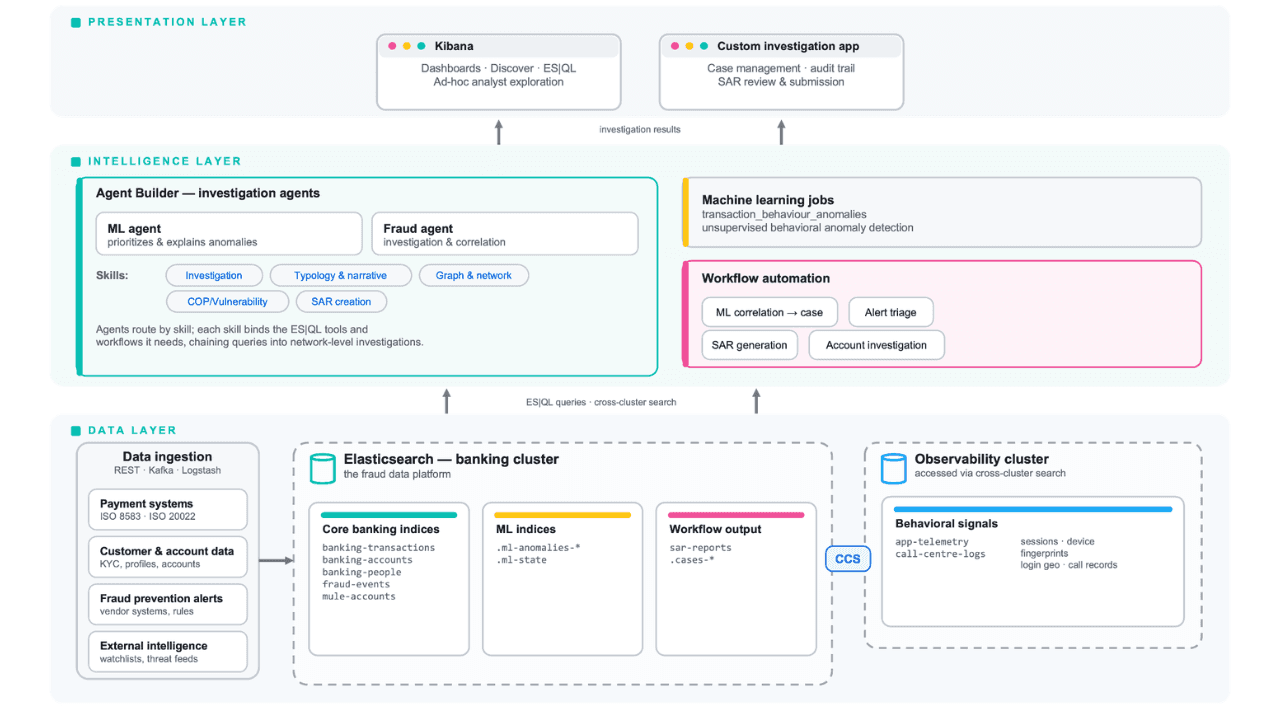
Follow the money: tracing laundering networks with ES|QL and cross-cluster search
The data model, cross-cluster architecture and five ES|QL queries that power mule detection and laundering network tracing, built from infrastructure most financial institutions already run.