Get hands-on with Elasticsearch: Dive into our sample notebooks in the Elasticsearch Labs repo, start a free cloud trial, or try Elastic on your local machine now.
Two new Elasticsearch ES|QL processing commands, METRICS_INFO and TS_INFO, tell you which metrics and time series actually have data for your current query context, not just what the mapping declares. Field mappings enumerate every field ever written; these commands return what's actively ingested, typed, and queryable right now, scoped to your time window and filters. A single-line query against 1.84 billion documents and 1.4 million time series returns in ~4 seconds. Available GA in Elasticsearch 9.4 and Elastic Cloud Serverless.
Why time series discovery matters
Elasticsearch uses time series data streams (TSDS) to efficiently store metrics. Backed by a fully columnar store, metrics stored in TSDS in Elasticsearch 9.4 require up to 17x less storage compared to using a standard index. Starting with Elasticsearch 9.2, we've also added time-series support in Elasticsearch Query Language (ES|QL) as a fully supported capability when querying data stored in TSDS.
If you operate TSDS in Elasticsearch, you already know the pattern: dimensions identify a series, metrics carry typed values like gauge or counter, and the TS source command in ES|QL enables time series aggregation functions such as RATE and AVG_OVER_TIME.
What that pipeline can't tell you (but you need to know just as often) is which metrics and time series actually exist right now, for the slice of data you care about. Field mappings enumerate every field that was ever declared; they don't show what's actively being ingested in a specific cluster, environment, or time window. That gap shows up across very different workflows:
- Dashboard building. Metric and dimension pickers should reflect what the cluster currently holds for the user's filters, not every field that has ever been mapped. Otherwise, dropdowns stay cluttered with stale options and panels render empty.
- Onboarding to an unfamiliar TSDS. A new cluster, a new integration, a customer's data. A quick list of the metrics being ingested, with their types, units, and applicable dimensions, replaces hours of mapping spelunking and ad hoc probe queries.
- Data quality investigations. Mapping drift (the same metric declared
gaugein one backing index andcounterin another) and dimension-cardinality explosions both surface immediately in the catalog output. - Query validation. Before running an expensive
TS ... | STATSaggregation, confirm that the metric and dimensions you're about to use really have data in your window.
Kibana already relies on this internally. The dynamic metrics catalog in the observability experience appends METRICS_INFO to the user's active TS query so the UI only offers metrics that truly exist for the current filters, rather than every field in the mapping.
The problem: Mappings are an inventory of fields, not time series
Operations teams routinely need answers to questions that mapping APIs alone cannot answer:
- Which metrics actually have data in this environment, for this cluster, in this time range?
- How are those metrics typed, and which dimensions apply when building or validating a query?
- How many distinct time series exist per metric?
Until now, answering these questions meant piecing together mapping APIs, ad hoc queries, and guesswork. METRICS_INFO and TS_INFO turn those questions into single-line ES|QL queries that fit naturally into the same pipeline you use for STATS:
| metric_name | data_stream | unit | metric_type | field_type | dimension_fields |
|---|---|---|---|---|---|
| network.eth0.rx | k8s | packets | gauge | integer | [cluster, pod, region] |
| network.eth0.tx | k8s | packets | gauge | integer | [cluster, pod, region] |
| network.total_bytes_in | k8s | bytes | counter | long | [cluster, pod, region] |
| network.total_cost | k8s | usd | counter | double | [cluster, pod, region] |
How these commands integrate with ES|QL pipelined queries
Both commands are processing commands. Once you run one, the table is replaced: Downstream commands, like KEEP, WHERE, or STATS, operate on metadata rows, not the original time series documents.
A few rules to keep in mind:
- They apply only after a
TSsource. Using them afterFROMor without a precedingTSsource produces an error. - They must appear before
STATS,SORT, orLIMITrun on the time series rows returned byTS. For example,TS ... | STATS ... | METRICS_INFOis invalid;TS ... | METRICS_INFO | STATS ...is valid becauseSTATSthen runs on the metadata table. - You can filter and aggregate after
METRICS_INFOorTS_INFOon the metadata columns with the usual processing commands. - You can include filters before them, for example, narrowing by
@timestampor dimensions, so that the produced metadata reflects series that match your query context, not the entire index.
Conceptually, the pipeline looks like this:
This design means you can scope a catalog to exactly the slice of data you care about and then post-process the result with more ES|QL commands as desired.
How to use METRICS_INFO and TS_INFO in practice
METRICS_INFO retrieves information about the metrics available in your time series data streams, together with applicable dimensions and other metadata, all scoped to the current TS query. TS_INFO does the same for individual time series. Each row is one metric plus the dimension values that identify one series.
Each command offers a different view to time series metadata: METRICS_INFO collapses what you see into one row per distinct metric signature: the metric name plus how it's declared (type, unit, field type, which dimension fields apply) as observed across backing indices. TS_INFO adds one row per metric and time series, with a dimensions column that holds the concrete label set for each series, formatted as a JSON object (for instance, {"job":"elasticsearch","instance":"instance_1"}).
If the same logical metric name shows up with incompatible metadata in different places, you get multiple rows or multi-valued cells. That's a useful signal when you're tracking down mapping drift.
Both commands expose the same core columns; only TS_INFO adds dimensions.
| Column | Meaning |
|---|---|
| metric_name | Name of the metric. |
| data_stream | Data stream(s) that contain this metric; multi-valued when it spans multiple data streams. |
| unit | Unit declared in the mapping (e.g. bytes); multi-valued when definitions differ across backing indices; may be null. |
| metric_type | Types such as gauge or counter; multi-valued when definitions differ across backing indices. |
| field_type | Elasticsearch field type (long, double, ...); multi-valued when definitions differ across backing indices. |
| dimension_fields | Dimension field names for this metric (multi-valued): the union of dimension keys across all time series for that metric. |
| dimensions | TS_INFO only. JSON-encoded dimension key/value pairs that identify one time series. |
Start with a catalog of names and types. The smallest useful query is a TS source, METRICS_INFO, and a sort so the table is easy to scan:
| metric_name | data_stream | unit | metric_type | field_type | dimension_fields |
|---|---|---|---|---|---|
| network.eth0.rx | k8s | packets | gauge | integer | [cluster, pod, region] |
| network.eth0.tx | k8s | packets | gauge | integer | [cluster, pod, region] |
| network.total_bytes_in | k8s | bytes | counter | long | [cluster, pod, region] |
| network.total_cost | k8s | usd | counter | double | [cluster, pod, region] |
You can post-process the result as usual in ES|QL. For instance, you can trim columns or filter on metadata before aggregating:
| metric_name | metric_type |
|---|---|
| network.eth0.rx | gauge |
| network.eth0.tx | gauge |
| network.total_bytes_in | counter |
| network.total_cost | counter |
To find how many distinct metric names match a pattern (not which series), combine METRICS_INFO with STATS:
| matching_metrics |
|---|
| 2 |
Document predicates before the catalog command narrow the processed time series to data samples that actually exist in your window. The metrics listed are those with matching data, not every field that has ever been mapped:
| metric_name | data_stream | unit | metric_type | field_type | dimension_fields |
|---|---|---|---|---|---|
| network.eth0.rx | k8s | packets | gauge | integer | [cluster, pod, region] |
| network.eth0.tx | k8s | packets | gauge | integer | [cluster, pod, region] |
| network.total_bytes_in | k8s | bytes | counter | long | [cluster, pod, region] |
| network.total_cost | k8s | usd | counter | double | [cluster, pod, region] |
Run the same scoped pipeline, but swap the middle command for TS_INFO, and the question shifts from “which metrics match” to “which time series identities match”. Each row is one metric plus one combination of dimension values; sort on metric_name and dimensions so related series group together:
| metric_name | data_stream | unit | metric_type | field_type | dimension_fields | dimensions |
|---|---|---|---|---|---|---|
| network.eth0.rx | k8s | packets | gauge | integer | [cluster, pod, region] | {"cluster":"prod","pod":"one","region":"[eu, us]"} |
| network.eth0.rx | k8s | packets | gauge | integer | [cluster, pod, region] | {"cluster":"prod","pod":"three","region":"[eu, us]"} |
| network.eth0.rx | k8s | packets | gauge | integer | [cluster, pod, region] | {"cluster":"prod","pod":"two","region":"[eu, us]"} |
| network.eth0.tx | k8s | packets | gauge | integer | [cluster, pod, region] | {"cluster":"prod","pod":"one","region":"[eu, us]"} |
| network.eth0.tx | k8s | packets | gauge | integer | [cluster, pod, region] | {"cluster":"prod","pod":"three","region":"[eu, us]"} |
| network.eth0.tx | k8s | packets | gauge | integer | [cluster, pod, region] | {"cluster":"prod","pod":"two","region":"[eu, us]"} |
| network.total_bytes_in | k8s | bytes | counter | long | [cluster, pod, region] | {"cluster":"prod","pod":"one","region":"[eu, us]"} |
| network.total_bytes_in | k8s | bytes | counter | long | [cluster, pod, region] | {"cluster":"prod","pod":"three","region":"[eu, us]"} |
| network.total_bytes_in | k8s | bytes | counter | long | [cluster, pod, region] | {"cluster":"prod","pod":"two","region":"[eu, us]"} |
| network.total_cost | k8s | usd | counter | double | [cluster, pod, region] | {"cluster":"prod","pod":"one","region":"[eu, us]"} |
| network.total_cost | k8s | usd | counter | double | [cluster, pod, region] | {"cluster":"prod","pod":"three","region":"[eu, us]"} |
| network.total_cost | k8s | usd | counter | double | [cluster, pod, region] | {"cluster":"prod","pod":"two","region":"[eu, us]"} |
That extra column can be used to deduce metric cardinality. Each TS_INFO row is one time series for a given metric, so grouping with STATS counts how many distinct time series exist per metric:
| series_count | metric_name |
|---|---|
| 9 | network.eth0.rx |
| 9 | network.eth0.tx |
| 9 | network.total_bytes_in |
| 9 | network.total_cost |
Choosing between them: Use METRICS_INFO when you want a compact inventory of metric names and types in the filtered TS context. Use TS_INFO when you need label combinations, per-metric series counts. In practice, skim with METRICS_INFO and then switch to TS_INFO when the answer depends on which dimensions apply, not just what metrics exist.
Under the hood: How the commands are executed
Both METRICS_INFO and TS_INFO run inside the same distributed ES|QL execution that powers any TS query. In addition to standard features, like shard-level parallelism, Lucene filter pushdown, and coordinator-side merging, special care has been taken during implementation so that the cost scales with the number of matching time series, not the number of documents. Here's how each output row gets produced:
1. The TS command defines the scope. TS resolves your data stream pattern to its TSDS backing indices and turns any filters you place before the catalog command, such as a time range on @timestamp or dimension predicates in WHERE, into a Lucene query that runs on every shard that can match. Shards in backing indices outside the time window are pruned up front and never touched.
2. Each shard iterates over matching documents and tracks one per series. A TSDS index is physically sorted by _tsid first, then by @timestamp (descending). That sort matters here: All documents belonging to the same time series sit next to each other on disk, so as a shard processes documents in order, it only needs to keep the first document it sees for each new _tsid and skip the rest. The result is one representative document per time series that has at least one document matching your filters.
3. The mapping tells us what each field is. The backing index mapping is the source of truth for the metadata that describes each field:
- Fields declared with
time_series_metricare metrics, and the mapping carries each metric'smetric_type,field_type, and (if declared)meta.unit.
4. Synthetic source fills in the actual dimension and metric presence. For the one representative document per series, the shard reads a subset of _source containing only the dimension (and metric) paths the mapping declares. TSDS uses synthetic _source, so that subset is reconstructed primarily from doc values — no stored _source is needed. From that reconstructed sliver of JSON, the shard learns two things:
- The dimension key/value pairs for this series (the
dimensionsJSON forTS_INFO, and the set of dimension keys that feeddimension_fieldsfor both commands). - Which metric fields actually have data for this series in this backing index.
5. Partial aggregation happens inside each shard. Shards don't ship raw per-series rows upstream. They partially aggregate first, which is a big part of why catalog queries stay cheap.
6. The coordinator merges across shards and data streams. Each data node first reduces its own shards' partial results and streams them to the coordinator, which applies the same merge logic one more time.
7. The rest of the pipeline runs as usual. Everything after the catalog command (KEEP, WHERE, STATS, SORT, LIMIT) runs against this consolidated metadata table on the coordinator, exactly like any other ES|QL stage.
The net effect is that catalog queries do just enough work to identify one representative document per series, read a small reconstructed slice of that document, classify its fields against the mapping, and fold the results into a handful of metadata rows. Because the output cardinality is bounded by the number of matching series (for TS_INFO) or by the number of distinct metric signatures (for METRICS_INFO), not by the number of documents in the window, these commands stay responsive even against long retention windows and high-ingest data streams.
Running these commands against the full high cardinality TSDB benchmark corpus without a time range filter (1.84 B documents / 1.4 M time series / 2.77 TB uncompressed) on a single-node Elasticsearch (AWS c8gd.8xlarge, 24 cores, 24 GiB heap, NVMe SSD, 3 primary shards, force-merged), METRICS_INFO returns in ~4 seconds.
Beyond ad hoc queries
These commands also support product workflows inside Kibana. The UI appends METRICS_INFO to a user's TS query (when the query doesn't already include STATS) to build a metric catalog aligned with the user's filters, rather than relying solely on mappings.
These new commands are also the foundation of Prometheus-compatible metadata APIs we're adding to Elasticsearch, which Prometheus-based tools can use. Stay tuned for a dedicated blog post that goes into more detail.
Data quality
Multi-valued unit, metric_type, or field_type in the METRICS_INFO output, is a concise warning that backing indices aren't aligned on a metric's definition. TS_INFO makes it easier to see whether an explosion in cardinality comes from a handful of metrics or from dimension cardinality you should account for in alerts and aggregations. For example, ranking metrics by series count surfaces outliers at a glance:
| series_count | metric_name |
|---|---|
| 12000 | network.eth0.rx |
| 9 | network.eth0.tx |
| 9 | network.total_bytes_in |
| 9 | network.total_cost |
When a single metric dwarfs the rest, as network.eth0.rx does above, the explosion is concentrated in a handful of metrics, and inspecting that metric's dimensions pinpoints which label is growing. Comparable counts across metrics instead point at shared dimension cardinality, such as a newly introduced pod or instance value propagating through every time series.
Availability
METRICS_INFO and TS_INFO are generally available in Elastic Cloud Serverless and in Elasticsearch basic starting with the 9.4.0 release.
For command pages (syntax, restrictions, and examples), see METRICS_INFO and TS_INFO.
For background on TSDS and the TS command itself, start with the official documentation on time series data streams and the TS source command.
Pour aller plus loin
How to build search analytics on Elastic using OpenTelemetry, no extra pipeline required
How to instrument your search application to use modern Open Telemetry standard to drive insights in to your search and users.
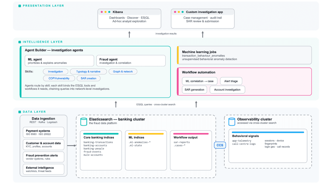
Follow the money: tracing laundering networks with ES|QL and cross-cluster search
The data model, cross-cluster architecture and five ES|QL queries that power mule detection and laundering network tracing, built from infrastructure most financial institutions already run.

1 juillet 2026
One command. Natural language. Your Elasticsearch data, straight to the terminal.
Query your Elasticsearch data from the terminal in plain English. The official Elastic GitHub Copilot CLI plugin generates and runs ES|QL queries against your cluster. No Kibana, no manual syntax.
30 juin 2026
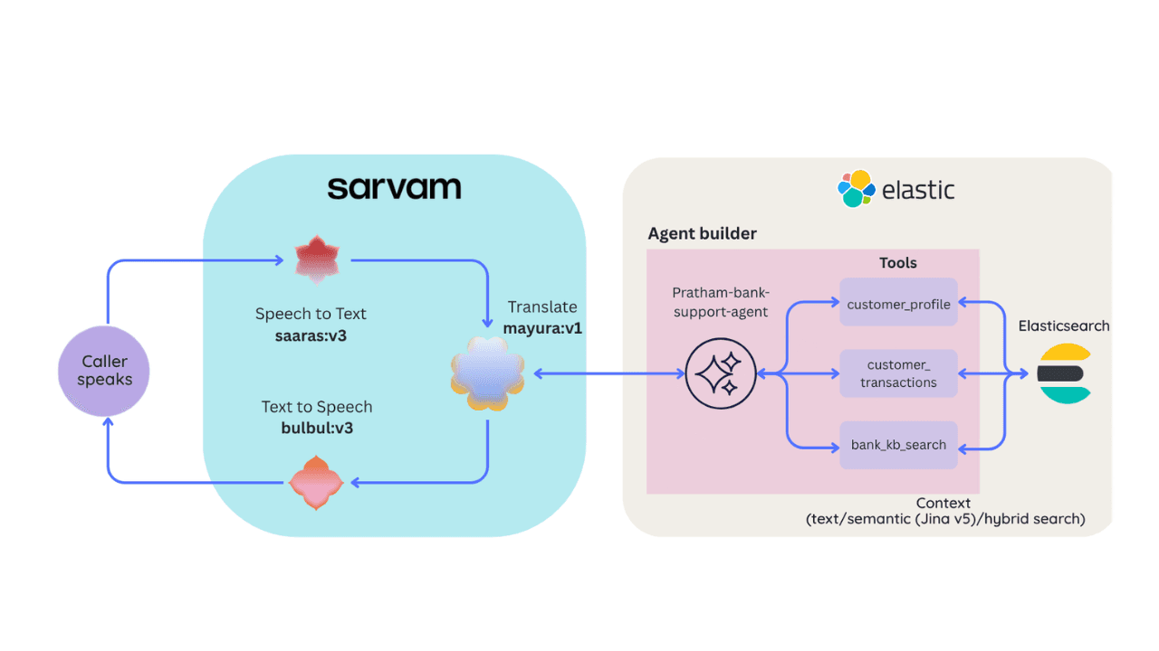
Building a multilingual voice agent with Elastic Agent Builder & Sarvam AI
A working demo combining Sarvam AI speech with Elastic Agent Builder: identity verification, per-customer ES|QL queries, and mid-call language switching across 22 Indian languages without multilingual indices.

29 juin 2026
Bringing it together: How we rebuilt Elasticsearch as a columnar metrics engine; 6.6x less storage, 160x faster queries
Elasticsearch metrics in version 9.4 run on a fully columnar engine: 6.6x less storage, 160x faster queries, native PromQL and OTel support.