Interpreting multi-bucket impact anomalies using Elastic machine learning features
You may have noticed that sometimes the anomaly results you get from our anomaly detector are marked with crosses instead of circles. These crosses indicate a special type of anomaly: a multi-bucket impact anomaly. We first introduced these new types of results in our blog post on the 6.5 release. In short, this means that the anomaly was not due to a single anomalous value in the current bucket, but rather to an anomalous sequence of values in the previous 12 buckets. The values themselves may not be unusual and may even be within the model bounds, but in a sequence they make up an anomalous progression of values with respect to the history of the dataset.
Let’s take a closer look at these anomalies to understand them better.
Why are multi-bucket anomalies useful?
A key requirement for using ML anomaly detection in the Elastic Stack is deciding on a bucket span. This value determines the granularity at which our anomaly detection algorithms observe and alert on the data. What happens if we have a dataset where anomalies usually occur on a five-minute range, but we are also interested in detecting anomalies that occur on a longer time range? For example, we would like to be alerted in sudden drops in visitor count over a five-minute range, but would also want to know if we experience consecutive drops in visitor counts over an hour. This is where multi-bucket anomalies come in handy. Instead of focusing on single anomalous buckets, multi-bucket anomalies alert us to the presence of anomalous regions of time where multiple sequential buckets exhibit unusual behavior. If you look back to the blog post we published with our 6.5 release, we showed how the introduction of multi-bucket impact anomalies allowed us to detect deviations from a usual pattern in a timeseries.
How do I interpret multi-bucket anomalies?
In order to understand why your dataset contains a multi-bucket anomaly, look at the behavior of the data in the last 12 bucket spans. To illustrate some of the concepts discussed in this blog post, we will be using an example dataset that illustrates the aggregate number of requests a company’s server receives. Let’s take a moment to look at the general characteristics of this dataset in Figure 1. The dataset exhibits a periodic weekly pattern as well as a daily pattern.
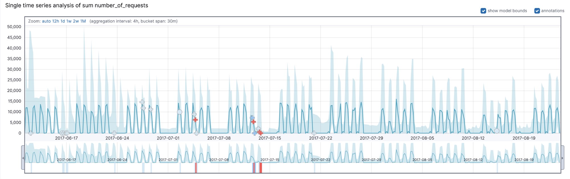
As one might expect, there are two temporal patterns that are immediately obvious: a daily pattern exhibiting high activity between 7am and 7pm and a weekly pattern exhibiting spikes of activity that correspond to the five working days with low to zero activity on the weekends. In addition to the variations at different times during the day and weekly variations, there are also hourly variations.
Suppose we want to take a very granular view of this data and set the bucket span to be 30 minutes. This will mean we will detect anomalies that occur on a 30-minute bucket timescale. But, we might also be interested in detecting things on a broader timescale — say we might be interested in days that are unusual or weeks that are unusual.
This is a prime use case for multi-bucket impact anomalies — we will run a machine learning job that detects anomalies in the count of requests sent to the company’s server with a 30-minute bucket span, which will provide insights into anomalies that occur on short time scales, while also detecting unusual periods of up to 6 hours (12 buckets * 30 minutes). To show some subtle effects that multi-bucket impact anomalies introduce into machine learning jobs with “sided” configurations (high_* or low_* detectors), we will also run the same job with a low_count and a high_count detector and compare the differences in the results in the following sections of this post.
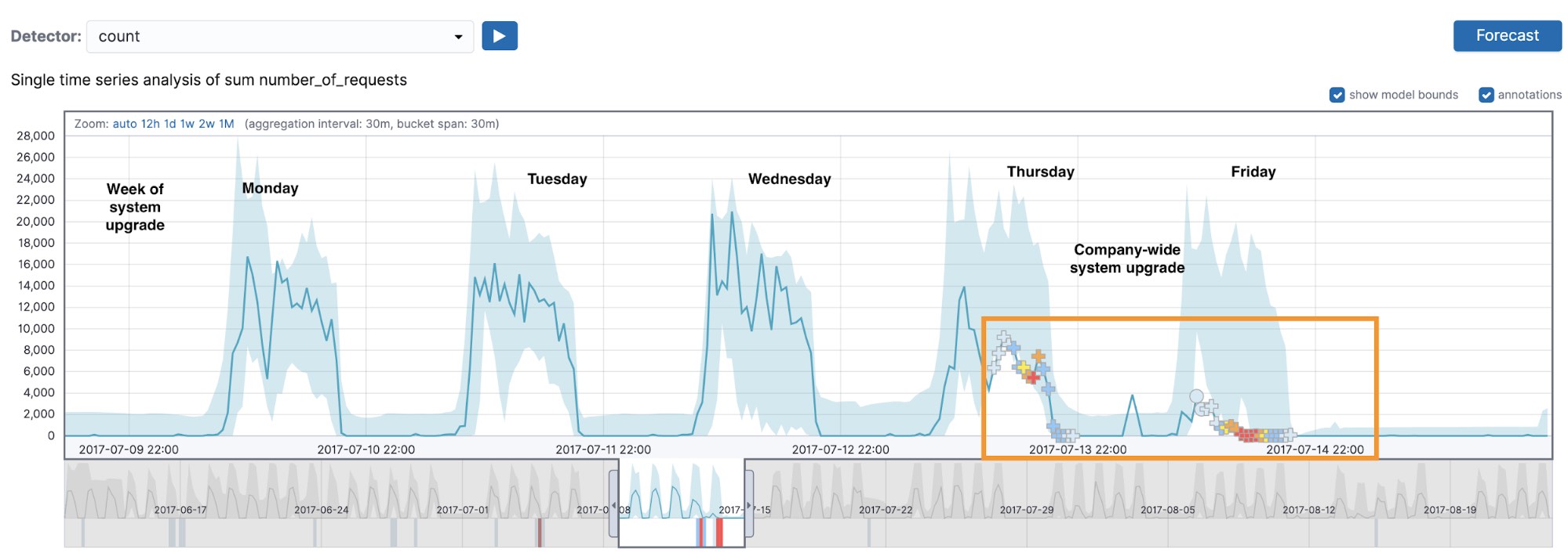
Let’s take a look at what the count detector was able to find in our dataset. As we can see from Figure 2, something strange took place during the working week starting on Monday 2017-07-10. During a system upgrade (which started on Thursday afternoon and continued well into Friday), there was an outage, which is detected as a series of multi-bucket impact anomalies (marked with crosses in the UI). The activity profiles on Thursday and Friday differ from those of a typical working week.
Zooming in to a section of time on Friday (Figure 3), we can see that in the 12 bucket period including and preceding the anomaly annotated with A, the values on each bucket are trailing below the midpoint of the model bounds, which is an approximate indicator of how we decide whether or not to mark something as a multi-bucket impact anomaly.
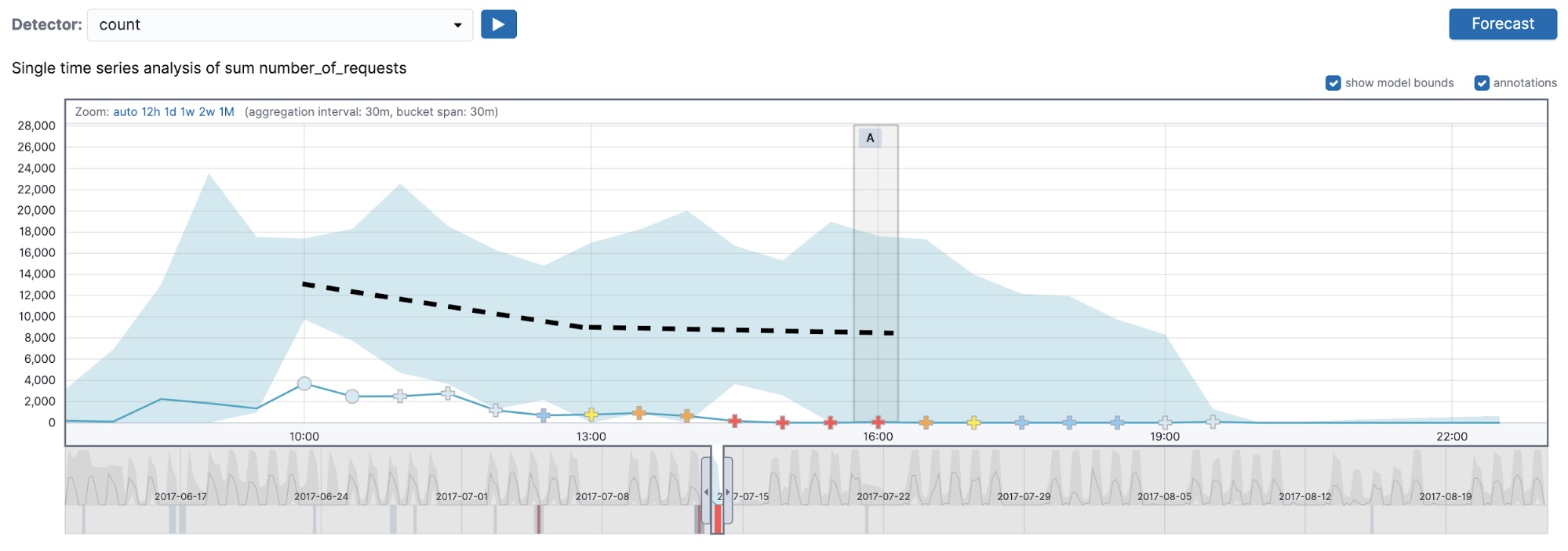
Another thing to observe is that the multi-bucket impact anomalies can occur on values that are within model bounds — sometimes even on values that are very close to the typical value observed for this region of the data. This, while counterintuitive, is a possible scenario, since we are alerting on an anomalous region instead of an anomalous bucket. It might not be too unusual to observe one bucket value that is slightly higher than is typical, but if we observe several buckets in a row, where the values are slightly higher than is typical, this could be a potential anomalous region to be investigated.
Thus when you are examining multi-bucket impact results, it is important to bear in mind that these results are for a region of buckets instead of a single bucket and adjust your investigations accordingly.
Finally, it’s good to note that when the multi-bucket anomaly detection algorithm examines a sequence of buckets, it gives more weight to the buckets that are closer in time to the bucket it is analyzing.
Do multi-bucket impact anomalies respect high_* and low_* sided detectors?
A common point of confusion when interpreting multi-bucket impact anomalies concerns their behaviors with sided detectors (for example a high_count or a low_count detector). Let’s examine an anomalous region picked out by the high_count detector with a 30-minute bucket span (see Figure 4).
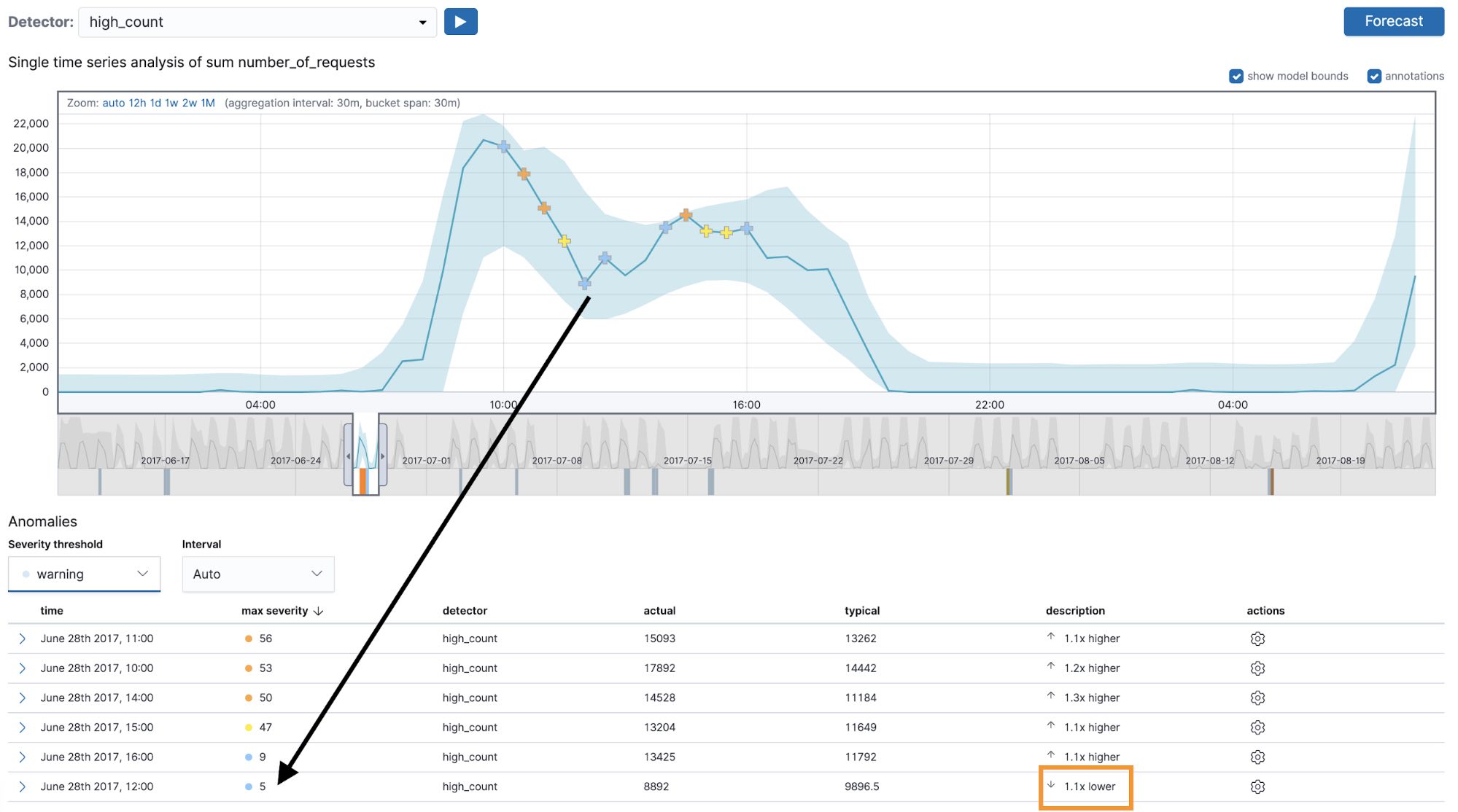
The first thing to notice here is the anomaly occurs when the actual value dips below the typical value for this region of the data. This may seem counterintuitive. After all, our anomaly detector was configured using the high_count function, so it should be looking for anomalies where the actual value exceeds the typical. This would indeed be true for regular anomalies, but not for multi-bucket anomalies. Since the latter depend on the observed values in multiple buckets as opposed to a single bucket, it is possible to be alerted about an anomalous region even if the actual value in the bucket where the multi-bucket anomaly is marked is below the typical.
We do, however, respect the side (high_* or low_*) of the detector in the region as a whole. We would only mark something as a multi-bucket impact anomaly if the values of the buckets in the region as a whole were higher than usual. If you examine the anomaly marked with a black arrow in Figure 4, you will notice that the actual value in the current bucket is lower than the typical, yet the preceding buckets contain values that are above the midpoint of the model bounds, which leads the high_count detector to mark this as an anomalous region in time. In summary, this means that the region can contain individual buckets where the actual value is lower than typical (see the highlighted bucket in Figure 4).
In the UI, the multi-bucket impact anomalies are marked with crosses in the charts but the same symbol is not carried over into the anomaly results table (as you can see in Figure 4 — the same anomaly is marked with a cross in the UI and with a circle in the chart). To view the multi-bucket impact in the anomaly results table, you can expand the row, which may not be obvious to first-time users.
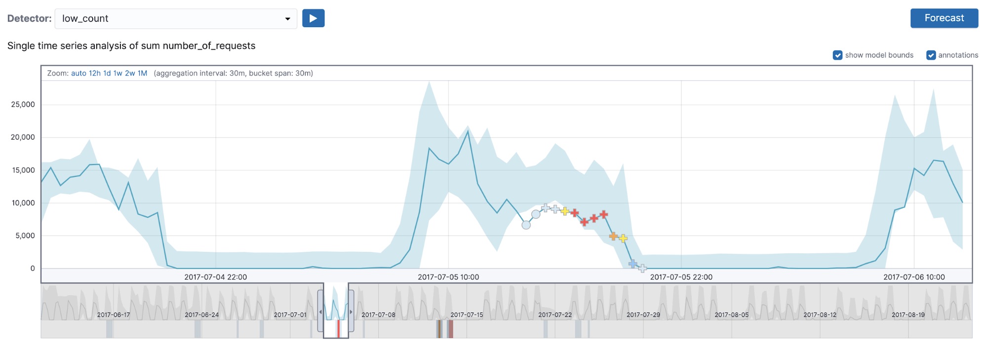
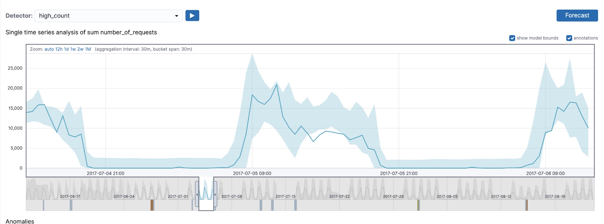
An example that displays that multi-bucket impact anomalies do respect detector side is shown in Figure 5. In this figure, we are displaying the results of the low_count and high_count detectors (both with a 30-minute bucket span) on July 5th, 2017.
As you can see from Figure 5, the low_count detector detects a series of multi-bucket impact anomalies, but in the high_count detector we no longer detect those, because in the region of interest the bucket values are on average lower than typical and thus our high_* sided detector will not pick those up. Even though multi-bucket impact anomalies can occur on buckets where the individual bucket value is on the wrong side of the detector (that is, a lower-than-typical value marked as anomalous in a high_* detector), the region flagged by the multi-bucket anomaly on the whole respects the sidedness of the detector.
How are multi-bucket impact anomalies scored?
If you examine multi-bucket impact anomalies in the UI, you will notice that they are graded from high multi-bucket impact to low multi-bucket impact. If you are using the API to retrieve machine learning results, multi-bucket impact anomalies will have a multi_bucket_impact field, which will score the anomaly from –5 to 5. Anomalies with a multi_bucket_impact value of greater than or equal to 2 are considered multi-bucket impact anomalies and are marked with crosses in our UI. This score is independent of the anomaly score, which determines the severity of the alert and thus the colour of the multi-bucket impact cross in the UI.
To further understand how we compute this score, consider the following. Every single bucket of data we examine with our anomaly detector can be anomalous in two ways: as part of a sequence of buckets that make up an anomalous region in time or on its own as a single bucket. For each bucket of data we examine, we compute two probabilities. The first probability captures the likelihood of observing a bucket value as extreme or more extreme based on the model of the data we have built up until this point in time. The second probability is based on a model of a multi-bucket feature — a kind of weighted average with a window of 12 buckets (the current bucket and the 11 buckets preceding it) that attempts to capture the anomalousness of a whole region the bucket is part of.
We then examine these probabilities in relation to one another. If both the single bucket and the multi-bucket probability are roughly on the same order of magnitude, we assign a multi-bucket impact score of 0 — that is, there is no significant contribution to this anomaly from the region of bucket preceding it. On the other hand, if the single bucket probability is high (that is, it is a value that is likely to occur based on our model of the series) and the multi-bucket impact probability is low (the bucket is part of an anomalous sequence of buckets that is very unlikely to occur), we would assign a high multi-bucket impact value to indicate that the anomalousness of this bucket results from an anomalous region of time as opposed to a single anomalous bucket value.
Conclusion
Multi-bucket impact anomalies were developed to give you two perspectives of your data: a granular perspective determined by your bucket span configuration, and a more zoomed-out view, which is able to pick out anomalies in longer periods of time. Therefore, a key thing to keep in mind when examining multi-bucket impact anomalies in your results is that they are referring to the anomalousness of a group of buckets in a region of time, instead of a single bucket and thus it is entirely possible for a multi-bucket anomaly to occur at a bucket value that is within model bounds or on a bucket value that is lower than typical for a detector designed to pick out values higher than typical (and vice versa).
Want to learn more? Check out our machine learning documentation. Or hop in and try it out yourself with a free 14-day trial of the Elasticsearch Service.