Finding outliers | Machine Learning in the Elastic Stack [8.3]

IMPORTANT: No additional bug fixes or documentation updates will be released for this version. For the latest information, see the current release documentation.

› ›

« Data frame analytics overview Predicting numerical values with regression »

Finding outliersedit

Outlier detection is identification of data points that are significantly different from other values in the data set. For example, outliers could be errors or unusual entities in a data set. Outlier detection is an unsupervised machine learning technique, there is no need to provide training data.

Outlier detection is a batch analysis, it runs against your data once. If new data comes into the index, you need to do the analysis again on the altered data.

Outlier detection algorithmsedit

In the Elastic Stack, we use an ensemble of four different distance and density based outlier detection methods:

distance of K^th nearest neighbor: computes the distance of the data point to its K^th nearest neighbor where K is a small number and usually independent of the total number of data points.
distance of K-nearest neighbors: calculates the average distance of the data points to their nearest neighbors. Points with the largest average distance will be the most outlying.
local outlier factor (lof): takes into account the distance of the points to their K nearest neighbors and also the distance of these neighbors to their neighbors.
local distance-based outlier factor (ldof): is a ratio of two measures: the first computes the average distance of the data point to its K nearest neighbors; the second computes the average of the pairwise distances of the neighbors themselves.

You don’t need to select the methods or provide any parameters, but you can override the default behavior if you like. Distance based methods assume that normal data points remain closer or similar in value while outliers are located far away or significantly differ in value. The drawback of these methods is that they don’t take into account the density variations of a data set. Density based methods are used for mitigating this problem.

The four algorithms don’t always agree on which points are outliers. By default, outlier detection jobs use all these methods, then normalize and combine their results and give every data point in the index an outlier score. The outlier score ranges from 0 to 1, where the higher number represents the chance that the data point is an outlier compared to the other data points in the index.

Feature influenceedit

Feature influence – another score calculated while detecting outliers – provides a relative ranking of the different features and their contribution towards a point being an outlier. This score allows you to understand the context or the reasoning on why a certain data point is an outlier.

1. Define the problemedit

Outlier detection in the Elastic Stack can be used to detect any unusual entity in a given population. For example, to detect malicious software on a machine or unusual user behavior on a network. As outlier detection operates on the assumption that the outliers make up a small proportion of the overall data population, you can use this feature in such cases. Outlier detection is a batch analysis that works best on an entity-centric index. If your use case is based on time series data, you might want to use anomaly detection instead.

The machine learning features provide unsupervised outlier detection, which means there is no need to provide a training data set.

2. Set up the environmentedit

Before you can use the Elastic Stack machine learning features, there are some configuration requirements (such as security privileges) that must be addressed. Refer to Setup and security.

3. Prepare and transform dataedit

Outlier detection requires specifically structured source data: a two dimensional tabular data structure. For this reason, you might need to transform your data to create a data frame which can be used as the source for outlier detection.

You can find an example of how to transform your data into an entity-centric index in this section.

4. Create a jobedit

Data frame analytics jobs contain the configuration information and metadata necessary to perform an analytics task. You can create data frame analytics jobs via Kibana or using the create data frame analytics jobs API. Select outlier detection as the analytics type that the data frame analytics job performs. You can also decide to include and exclude fields to/from the analysis when you create the job.

5. Start the jobedit

You can start the job via Kibana or using the start data frame analytics jobs API. An outlier detection job has four phases:

reindexing: documents are copied from the source index to the destination index.
loading_data: the job fetches the necessary data from the destination index.
computing_outliers: the job identifies outliers in the data.
writing_results: the job matches the results with the data rows in the destination index, merges them, and indexes them back to the destination index.

After the last phase is finished, the job stops and the results are ready for evaluation.

Outlier detection jobs – unlike other data frame analytics jobs – run one time in their life cycle. If you’d like to run the analysis again, you need to create a new job.

6. Evaluate the resultsedit

Using the data frame analytics features to gain insights from a data set is an iterative process. After you defined the problem you want to solve, and chose the analytics type that can help you to do so, you need to produce a high-quality data set and create the appropriate data frame analytics job. You might need to experiment with different configurations, parameters, and ways to transform data before you arrive at a result that satisfies your use case. A valuable companion to this process is the evaluate data frame analytics API, which enables you to evaluate the data frame analytics performance. It helps you understand error distributions and identifies the points where the data frame analytics model performs well or less trustworthily.

To evaluate the analysis with this API, you need to annotate your index that contains the results of the analysis with a field that marks each document with the ground truth. The evaluate data frame analytics API evaluates the performance of the data frame analytics against this manually provided ground truth.

The outlier detection evaluation type offers the following metrics to evaluate the model performance:

confusion matrix
precision
recall
receiver operating characteristic (ROC) curve.

Confusion matrixedit

A confusion matrix provides four measures of how well the data frame analytics worked on your data set:

True positives (TP): Class members that the analysis identified as class members.
True negatives (TN): Not class members that the analysis identified as not class members.
False positives (FP): Not class members that the analysis misidentified as class members.
False negatives (FN): Class members that the analysis misidentified as not class members.

Although, the evaluate data frame analytics API can compute the confusion matrix out of the analysis results, these results are not binary values (class member/not class member), but a number between 0 and 1 (which called the outlier score in case of outlier detection). This value captures how likely it is for a data point to be a member of a certain class. It means that it is up to the user to decide what is the threshold or cutoff point at which the data point will be considered as a member of the given class. For example, the user can say that all the data points with an outlier score higher than 0.5 will be considered as outliers.

To take this complexity into account, the evaluate data frame analytics API returns the confusion matrix at different thresholds (by default, 0.25, 0.5, and 0.75).

Precision and recalledit

Precision and recall values summarize the algorithm performance as a single number that makes it easier to compare the evaluation results.

Precision shows how many of the data points that were identified as class members are actually class members. It is the number of true positives divided by the sum of the true positives and false positives (TP/(TP+FP)).

Recall shows how many of the data points that are actual class members were identified correctly as class members. It is the number of true positives divided by the sum of the true positives and false negatives (TP/(TP+FN)).

Precision and recall are computed at different threshold levels.

Receiver operating characteristic curveedit

The receiver operating characteristic (ROC) curve is a plot that represents the performance of the binary classification process at different thresholds. It compares the rate of true positives against the rate of false positives at the different threshold levels to create the curve. From this plot, you can compute the area under the curve (AUC) value, which is a number between 0 and 1. The closer to 1, the better the algorithm performance.

The evaluate data frame analytics API can return the false positive rate (fpr) and the true positive rate (tpr) at the different threshold levels, so you can visualize the algorithm performance by using these values.

Detecting unusual behavior in the logs data setedit

The goal of outlier detection is to find the most unusual documents in an index. Let’s try to detect unusual behavior in the data logs sample data set.

Verify that your environment is set up properly to use machine learning features. If the Elasticsearch security features are enabled, you need a user that has authority to create and manage data frame analytics jobs. See Setup and security.

Since we’ll be creating transforms, you also need manage_data_frame_transforms cluster privileges.

Create a transform that generates an entity-centric index with numeric or boolean data to analyze.

In this example, we’ll use the web logs sample data and pivot the data such that we get a new index that contains a network usage summary for each client IP.

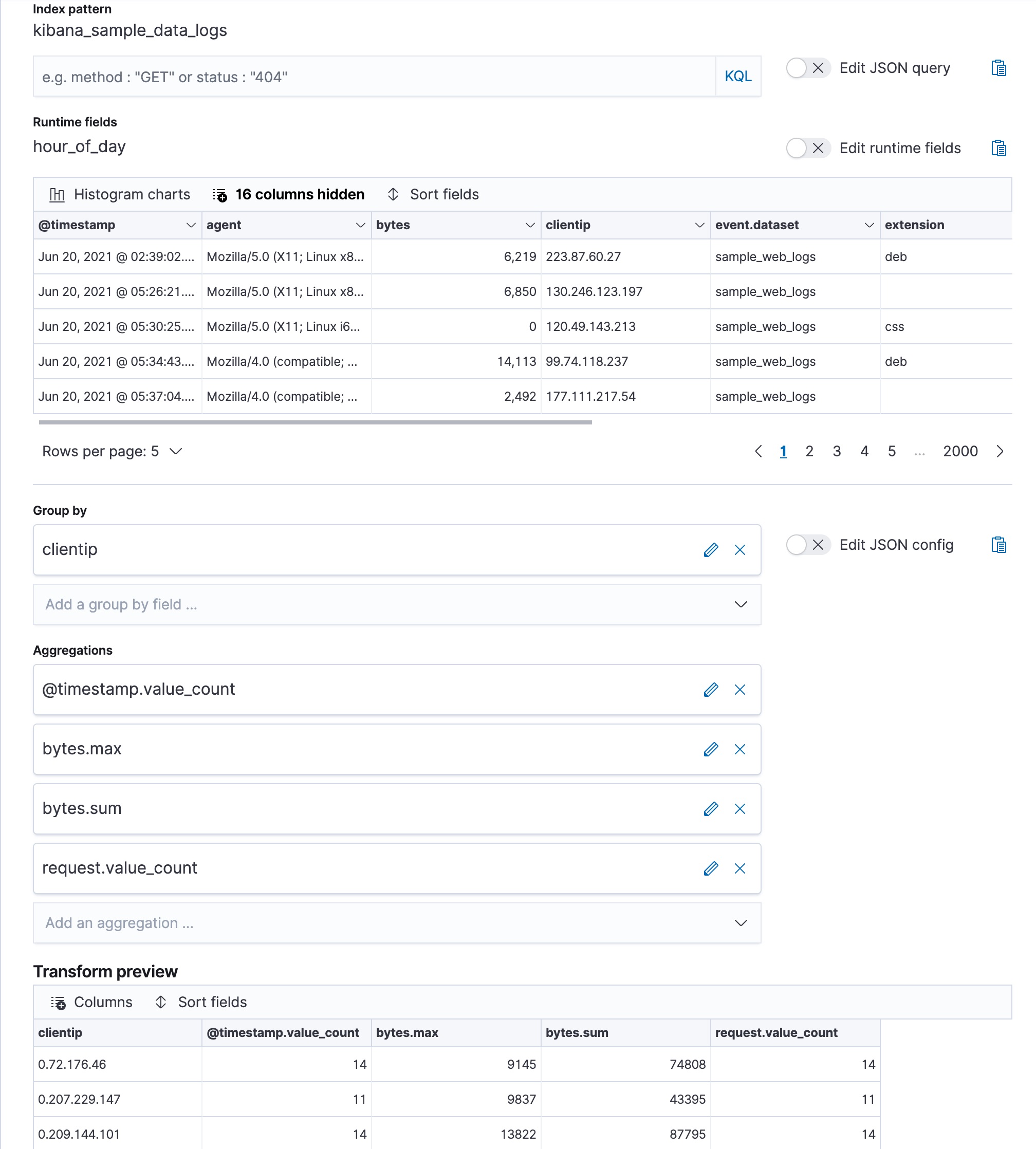
In particular, create a transform that calculates the number of occasions when a specific client IP communicated with the network (@timestamp.value_count), the sum of the bytes that are exchanged between the network and the client’s machine (bytes.sum), the maximum exchanged bytes during a single occasion (bytes.max), and the total number of requests (request.value_count) initiated by a specific client IP.

You can preview the transform before you create it in Stack Management > Transforms:

Alternatively, you can use the preview transform API and the create transform API.

API example

POST _transform/_preview
{
  "source": {
    "index": [
      "kibana_sample_data_logs"
    ]
  },
  "pivot": {
    "group_by": {
      "clientip": {
        "terms": {
          "field": "clientip"
        }
      }
    },
    "aggregations": {
      "@timestamp.value_count": {
        "value_count": {
          "field": "@timestamp"
        }
      },
      "bytes.max": {
        "max": {
          "field": "bytes"
        }
      },
      "bytes.sum": {
        "sum": {
          "field": "bytes"
        }
      },
      "request.value_count": {
        "value_count": {
          "field": "request.keyword"
        }
      }
    }
  }
}

PUT _transform/logs-by-clientip
{
  "source": {
    "index": [
      "kibana_sample_data_logs"
    ]
  },
  "pivot": {
    "group_by": {
      "clientip": {
        "terms": {
          "field": "clientip"
        }
      }
    },
    "aggregations": {
      "@timestamp.value_count": {
        "value_count": {
          "field": "@timestamp"
        }
      },
      "bytes.max": {
        "max": {
          "field": "bytes"
        }
      },
      "bytes.sum": {
        "sum": {
          "field": "bytes"
        }
      },
      "request.value_count": {
        "value_count": {
          "field": "request.keyword"
        }
      }
    }
  },
  "description": "Web logs by client IP",
  "dest": {
    "index": "weblog-clientip"
  }
}

For more details about creating transforms, see Transforming the eCommerce sample data.

Start the transform.

Even though resource utilization is automatically adjusted based on the cluster load, a transform increases search and indexing load on your cluster while it runs. If you’re experiencing an excessive load, however, you can stop it.

You can start, stop, and manage transforms in Kibana. Alternatively, you can use the start transforms API.
API example
```
POST _transform/logs-by-clientip/_start
```
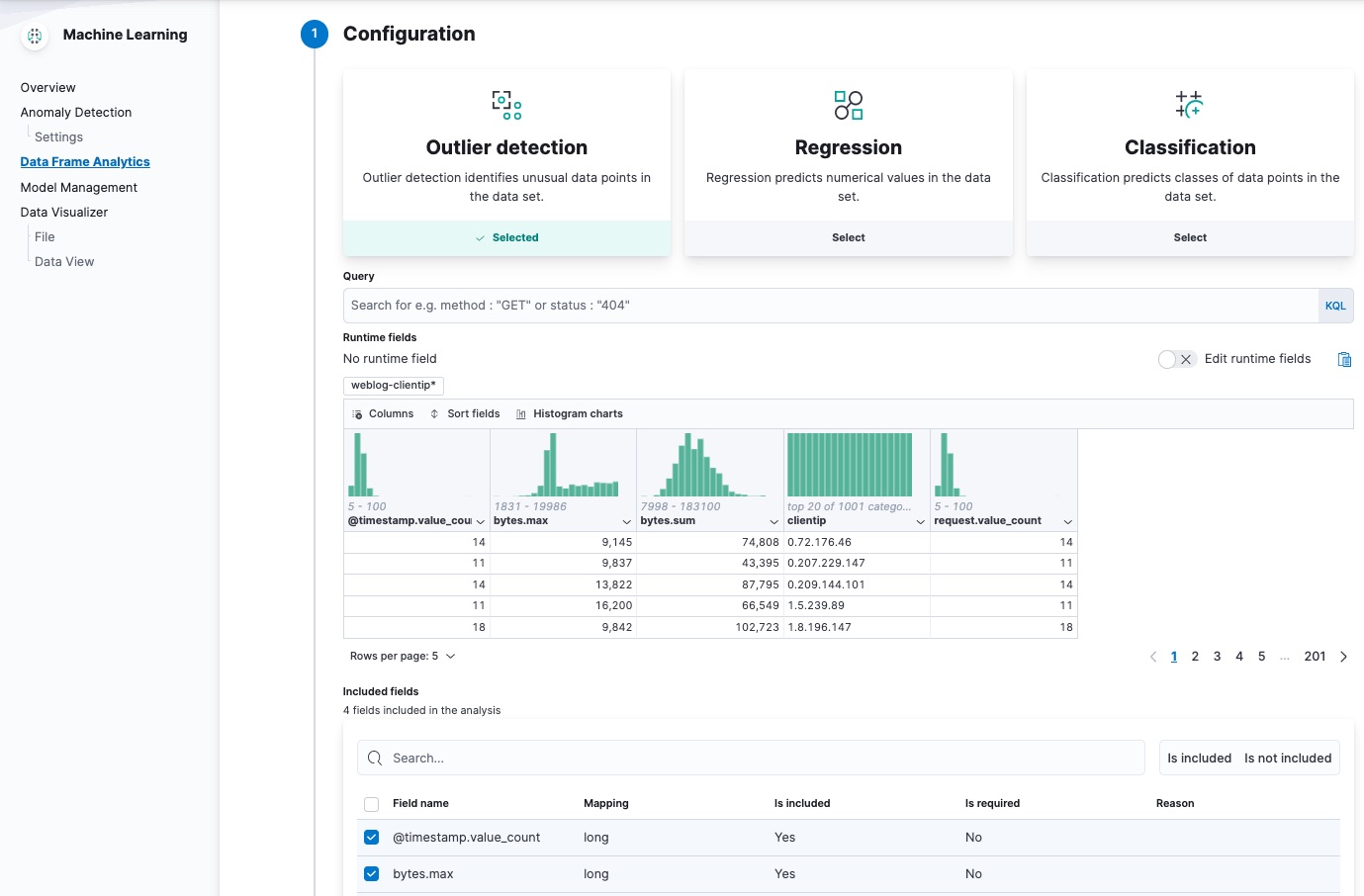
Create a data frame analytics job to detect outliers in the new entity-centric index.

In the wizard on the Machine Learning > Data Frame Analytics page in Kibana, select your new data view then use the default values for outlier detection. For example:

The wizard includes a scatterplot matrix, which enables you to explore the relationships between the fields. You can use that information to help you decide which fields to include or exclude from the analysis.

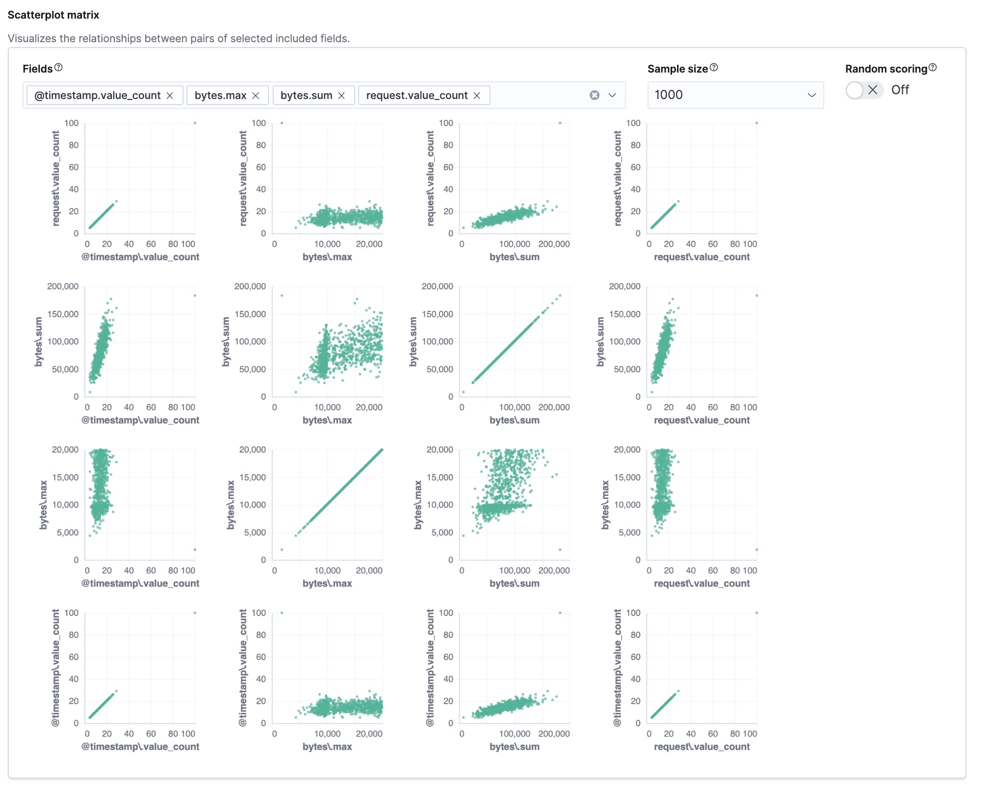
If you want these charts to represent data from a larger sample size or from a randomized selection of documents, you can change the default behavior. However, a larger sample size might slow down the performance of the matrix and a randomized selection might put more load on the cluster due to the more intensive query.

Alternatively, you can use the create data frame analytics jobs API.
API example
```
PUT _ml/data_frame/analytics/weblog-outliers
{
  "source": {
    "index": "weblog-clientip"
  },
  "dest": {
    "index": "weblog-outliers"
  },
  "analysis": {
    "outlier_detection": {
    }
  },
  "analyzed_fields" : {
    "includes" : ["@timestamp.value_count","bytes.max","bytes.sum","request.value_count"]
  }
}
```
After you configured your job, the configuration details are automatically validated. If the checks are successful, you can proceed and start the job. A warning message is shown if the configuration is invalid. The message contains a suggestion to improve the configuration to be validated.
Start the data frame analytics job.

You can start, stop, and manage data frame analytics jobs on the Machine Learning > Data Frame Analytics page. Alternatively, you can use the start data frame analytics jobs and stop data frame analytics jobs APIs.
API example
```
POST _ml/data_frame/analytics/weblog-outliers/_start
```
View the results of the outlier detection analysis.

The data frame analytics job creates an index that contains the original data and outlier scores for each document. The outlier score indicates how different each entity is from other entities.

In Kibana, you can view the results from the data frame analytics job and sort them on the outlier score:

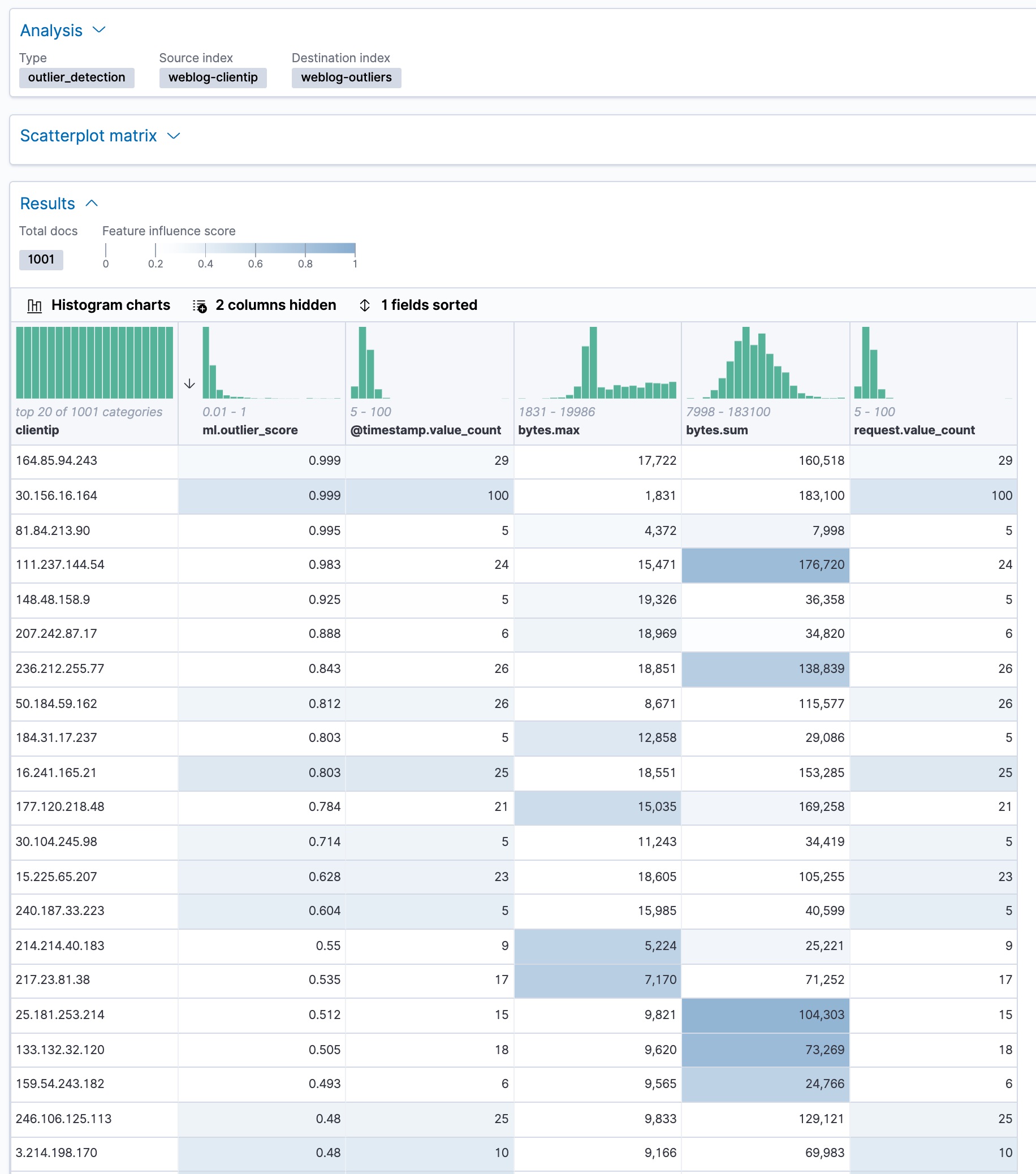
The ml.outlier score is a value between 0 and 1. The larger the value, the more likely they are to be an outlier. In Kibana, you can optionally enable histogram charts to get a better understanding of the distribution of values for each column in the result.

In addition to an overall outlier score, each document is annotated with feature influence values for each field. These values add up to 1 and indicate which fields are the most important in deciding whether an entity is an outlier or inlier. For example, the dark shading on the bytes.sum field for the client IP 111.237.144.54 indicates that the sum of the exchanged bytes was the most influential feature in determining that that client IP is an outlier.

If you want to see the exact feature influence values, you can retrieve them from the index that is associated with your data frame analytics job.
API example
```
GET weblog-outliers/_search?q="111.237.144.54"
```
The search results include the following outlier detection scores:
```
...
  "ml" : {
    "outlier_score" : 0.9830020666122437,
    "feature_influence" : [
      {
        "feature_name" : "@timestamp.value_count",
        "influence" : 0.005870792083442211
      },
      {
        "feature_name" : "bytes.max",
        "influence" : 0.12034820765256882
      },
      {
        "feature_name" : "bytes.sum",
        "influence" : 0.8679102063179016
      },
     {
        "feature_name" : "request.value_count",
        "influence" : 0.005870792083442211
      }
    ]
  }
...
```
Kibana also provides a scatterplot matrix in the results. Outliers with a score that exceeds the threshold are highlighted in each chart:

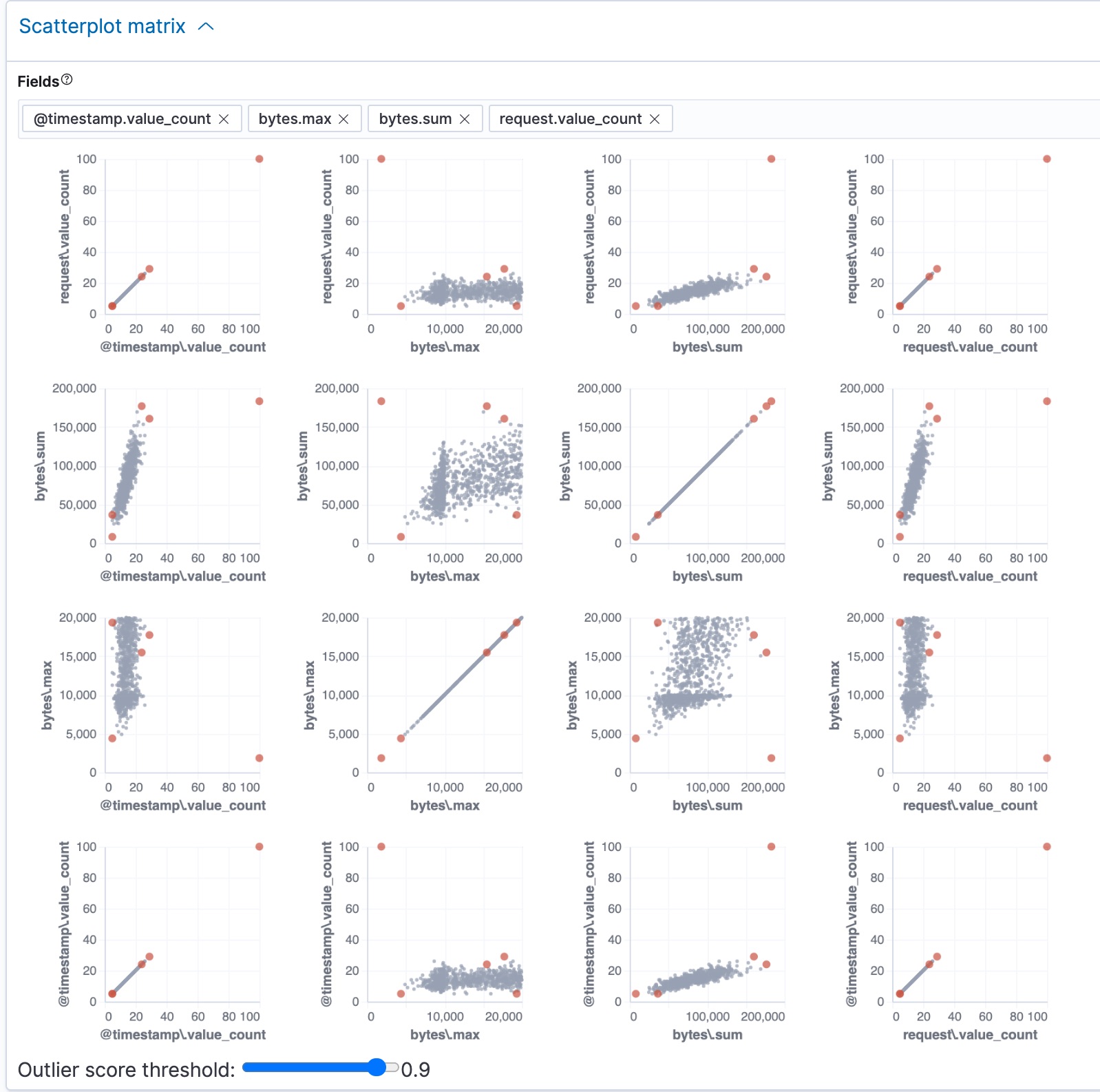
In addition to the sample size and random scoring options, there is a Dynamic size option. If you enable this option, the size of each point is affected by its outlier score; that is to say, the largest points have the highest outlier scores. The goal of these charts and options is to help you visualize and explore the outliers within your data.

Now that you’ve found unusual behavior in the sample data set, consider how you might apply these steps to other data sets. If you have data that is already marked up with true outliers, you can determine how well the outlier detection algorithms perform by using the evaluate data frame analytics API. See 6. Evaluate the results.

If you do not want to keep the transform and the data frame analytics job, you can delete them in Kibana or use the delete transform API and delete data frame analytics job API. When you delete transforms and data frame analytics jobs in Kibana, you have the option to also remove the destination indices and data views.

Finding outliersedit

Outlier detection algorithmsedit

Feature influenceedit

1. Define the problemedit

2. Set up the environmentedit

3. Prepare and transform dataedit

4. Create a jobedit

5. Start the jobedit

6. Evaluate the resultsedit

Confusion matrixedit

Precision and recalledit

Receiver operating characteristic curveedit

Detecting unusual behavior in the logs data setedit

Further readingedit