Visualizing France Salary Data with Region Maps in Kibana
Bonjour les amis. We're constantly adding new vector layers to our Elastic Maps Service. Most recently, we've added support for France department boundary vector layers to region maps. You may match results of terms in your Elasticsearch data to department names in either French or English. We have also included INSEE codes for each department as defined by Institut national de la statistique et des études économiques (INSEE) [National Institute of Statistics and Economic Studies]. INSEE collects, analyzes, and distributes information on the French economy and society.
#TalkPay
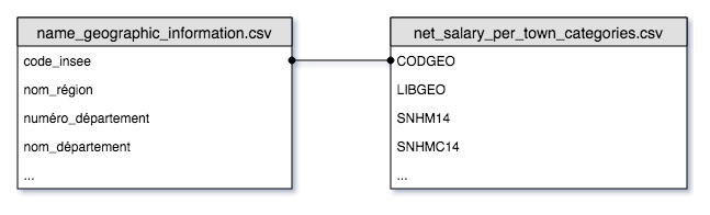
Kaggle has an interesting dataset from INSEE on employment, salaries, and population per town in France. We can import this dataset into Elasticsearch and visualize in Kibana region maps. For this project we will look at salary information.
Prepare the data
There are several data files in the Kaggle dataset that require a little massaging before we can import into Elasticsearch. The net_salary_per_town_categories.csv file includes a column called CODGEO which the dataset describes as the INSEE code for the Town. This can be joined to the code_insee column in the name_geographic_information.csv file. The name_geographic_information.csv file includes INSEE codes for the administrative regions, departments, and prefectures for each town. This normalization strategy works well for importing into relational databases, but we will want to join these tables (de-normalize) for importing into Elasticsearch.
SQLite is an incredibly useful and versatile database engine that we can use to join these tables. We’ll create a database file and import the CSV files into it.
sqlite3 france-salary.db
sqlite>.mode csv
sqlite>.import data/net_salary_per_town_categories.csv salary
sqlite>.import data/name_geographic_information.csv names
Let’s preview our data.
sqlite>.headers on
sqlite>SELECT * FROM salary LIMIT 5;
| CODGEO | LIBGEO | SNHM14 | SNHMC14 | ... |
| 01004 | Ambérieu-en-Bugey | 13.7 | 24.2 | ... |
| 01007 | Ambronay | 13.5 | 22.1 | ... |
| 01014 | Arbent | 13.5 | 27.6 | ... |
| 01024 | Attignat | 12.9 | 21.8 | ... |
| 01025 | Bâgé-la-Ville | 13 | 22.8 | ... |
sqlite>SELECT * FROM names LIMIT 5;
| code_insee | nom_commune | code_région | nom_région | ... |
| 1004 | Ambérieu-en-Bugey | 82 | Rhône-Alpes | ... |
| 1007 | Ambronay | 82 | Rhône-Alpes | ... |
| 1014 | Arbent | 82 | Rhône-Alpes | ... |
| 1024 | Attignat | 82 | Rhône-Alpes | ... |
| 1025 | Bâgé-la-Ville | 82 | Rhône-Alpes | ... |
Notice that the CODGEO column has a leading zero, but the code_insee column does not. This discrepancy appears in the CSV tables. In order to join the two tables, we’ll need to pad the code_insee column with a leading zero. We can do this with a little SQLite magic.
sqlite>CREATE TABLE names_ready as SELECT substr(‘00000’ || code_insee, -5, 5) as insee_town, * as FROM names;
sqlite>SELECT * FROM names_ready LIMIT 5;
| insee_town | code_insee | nom_commune | code_région | nom_région | ... |
| 01004 | 1004 | Ambérieu-en-Bugey | 82 | Rhône-Alpes | ... |
| 01007 | 1007 | Ambronay | 82 | Rhône-Alpes | ... |
| 01014 | 1014 | Arbent | 82 | Rhône-Alpes | ... |
| 01024 | 1024 | Attignat | 82 | Rhône-Alpes | ... |
| 01025 | 1025 | Bâgé-la-Ville | 82 | Rhône-Alpes | ... |
Now the insee_town column in the new names_ready table can be joined to the CODGEO column in the salary table. But first, let’s create indexes on those columns.
sqlite>CREATE INDEX idx_insee_town ON names_ready (insee_town);
sqlite>CREATE INDEX idx_codgeo ON salary (CODGEO);
Then we will create a table from a select query to join the salary and names tables and create useful aliases for the field names based on the metadata in the Kaggle dataset.
sqlite>CREATE TABLE france_salary as
    SELECT
    CODGEO as Town_INSEE,
    Nom_commune as Town_Name
    code_région as Region_INSEE,
    nom_région as Region_Name,
    numéro_département as Department_INSEE,
    nom_département as Department_Name,
    Préfecture as Prefecture_Name,
    Numéro_circonscription as Conscription_Number,
    Codes_postaux as Postal_Code,
    Latitude,
    Longitude,
    SNHM14 as mean_net_salary,
    SNHMF14 as mean_net_salary_female,
    SNHMH14 as mean_net_salary_male,
    SNHMC14 as mean_net_salary_hour_executive,
    SNHMFC14 as mean_net_salary_hour_executive_female,
    SNHMHC14 as mean_net_salary_hour_executive_male,
    SNHMP14 as mean_net_salary_hour_middlemanager,
    SNHMFP14 as mean_net_salary_hour_middlemanager_female,
    SNHMHP14 as mean_net_salary_hour_middlemanager_male,
    SNHME14 as mean_net_salary_hour_employee,
    SNHMFE13 as mean_net_salary_hour_employee_female,
    SNHMHE14 as mean_net_salary_hour_employee_male,
    SNHMO14 as mean_net_salary_hour_worker,
    SNHMFO14 as mean_net_salary_hour_worker_female,
    SNHMHO14 as mean_net_salary_hour_worker_male,
    SNHM1814 as mean_net_salary_hour_year18-25,
    SNHMF1814 as mean_net_salary_hour_year18-25_female,
    SNHMH1814 as mean_net_salary_hour_year18-25_male,
    SNHM2614 as mean_net_salary_hour_year26-50,
    SNHMF2614 as mean_net_salary_hour_year26-50_female,
    SNHMH2614 as mean_net_salary_hour_year26-50_male,
    SNHM5014 as mean_net_salary_hour_year50+,
    SNHMF5014 as mean_net_salary_hour_year50+_female,
    SNHMH5014 as mean_net_salary_hour_year50+_male
    FROM salary
    LEFT OUTER JOIN names_ready
    ON salary.CODGEO = names_ready.insee_town;
Ingest into Elasticsearch
Logstash is a great way to transform and ingest data for Elasticsearch. A multitude of plugins are available for Logstash. For this project we will use the CSV filter plugin to import data from a CSV file.
First, let’s generate a new CSV file called salary_data.csv from the table we created above.
sqlite>.headers on
sqlite>.mode csv
sqlite>.once salary_data.csv
sqlite>SELECT * from france_salary;
Next we’ll create a config file for Logstash to load this CSV file.
Here is our definition for the file input plugin. Change the path to the absolute path of your salary_data.csv file. Specifying /dev/null as the sincedb_path will ensure that Logstash always reads from the top of the file, but beware of this in production as it could create duplicate records.
input {
   file {
       path => "/path/to/france-salary/salary_data.csv"
       start_position => "beginning"
       codec => plain {
           charset => "UTF-8"
       }
       sincedb_path => "/dev/null"
   }
}
Then we must specify how to handle the CSV file using the CSV plugin. Columns in CSV files are always assumed to be text, so we need to use the convert parameter to change numeric fields into float for Elasticsearch.
filter {
   csv {
       separator => ","
       skip_header => "true"
       columns => [
           "Town_INSEE",
           "Town_Name",
           "Region_INSEE",
           "Region_Name",
           "Department_INSEE",
           "Department_Name",
           "Prefecture_Name",
           "Conscription_Number",
           "Postal_Code",
           "latitude",
           "longitude",
           "mean_net_salary",
           "mean_net_salary_female",
           "mean_net_salary_male",
           "mean_net_salary_hour_executive",
           "mean_net_salary_hour_executive_female",
           "mean_net_salary_hour_executive_male",
           "mean_net_salary_hour_middlemanager",
           "mean_net_salary_hour_middlemanager_female",
           "mean_net_salary_hour_middlemanager_male",
           "mean_net_salary_hour_employee",
           "mean_net_salary_hour_employee_female",
           "mean_net_salary_hour_employee_male",
           "mean_net_salary_hour_worker",
           "mean_net_salary_hour_worker_female",
           "mean_net_salary_hour_worker_male",
           "mean_net_salary_hour_year18_25",
           "mean_net_salary_hour_year18_25_female",
           "mean_net_salary_hour_year18_25_male",
           "mean_net_salary_hour_year26_50",
           "mean_net_salary_hour_year26_50_female",
           "mean_net_salary_hour_year26_50_male",
           "mean_net_salary_hour_year50over",
           "mean_net_salary_hour_year50over_female",
           "mean_net_salary_hour_year50over_male"
       ]
       convert => {
           "mean_net_salary" => "float"
           "mean_net_salary_female" => "float"
           "mean_net_salary_male" => "float"
           "mean_net_salary_hour_executive" => "float"
           "mean_net_salary_hour_executive_female" => "float"
           "mean_net_salary_hour_executive_male" => "float"
           "mean_net_salary_hour_middlemanager" => "float"
           "mean_net_salary_hour_middlemanager_female" => "float"
           "mean_net_salary_hour_middlemanager_male" => "float"
           "mean_net_salary_hour_employee" => "float"
           "mean_net_salary_hour_employee_female" => "float"
           "mean_net_salary_hour_employee_male" => "float"
           "mean_net_salary_hour_worker" => "float"
           "mean_net_salary_hour_worker_female" => "float"
           "mean_net_salary_hour_worker_male" => "float"
           "mean_net_salary_hour_year18_25" => "float"
           "mean_net_salary_hour_year18_25_female" => "float"
           "mean_net_salary_hour_year18_25_male" => "float"
           "mean_net_salary_hour_year26_50" => "float"
           "mean_net_salary_hour_year26_50_female" => "float"
           "mean_net_salary_hour_year26_50_male" => "float"
           "mean_net_salary_hour_year50over" => "float"
           "mean_net_salary_hour_year50over_female" => "float"
           "mean_net_salary_hour_year50over_male" => "float"
       }
   }
}
The hosts parameter in the output plugin section is the URL to your running Elasticsearch instance. We also specify stdout in json format as an output for debugging. The stdout parameters are not required for ingesting the data.
output {
   stdout {
codec => json
   }
   elasticsearch {
       hosts => ["localhost:9200"]
       index => "france-example-salary"
   }
}
Let’s call this file france-salary.conf and tell Logstash to use it for ingestion.
./bin/logstash -f /path/to/france-example-salary.conf
Logstash does not terminate automatically when it reaches the end of the file. Instead it will continue to monitor the CSV file for new data. Since we don’t expect to add more data to the CSV file you can safely stop Logstash using Ctrl-C when the output stops.
Create Maps of Salary by France Department
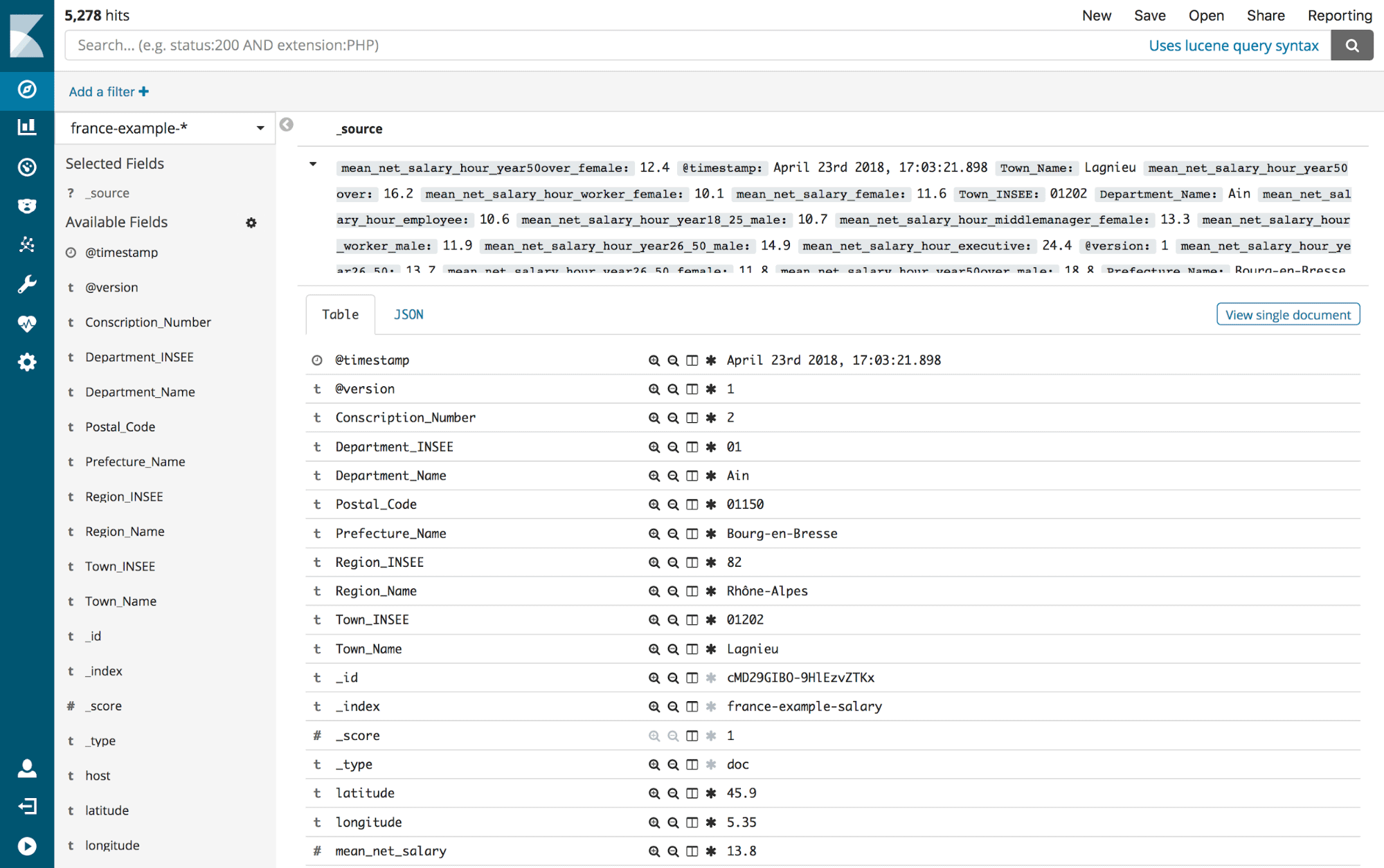
Create a new Index pattern in Kibana to match france-example-*. Then check out the Discover tab to make sure our data is there. It should look something like this.
Switch to the Visualize tab and create a new region map visualization using the france-example-* index. Set the value to average the mean_net_salary. The shape field should be a terms aggregation on the Department_Name keyword. This will average the mean_net_salary for all towns in each department. You may also want to set the size to large number (e.g. 100) in order to display all department data.
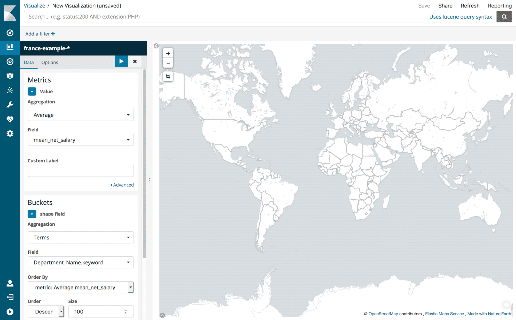
Nothing will appear on the map yet because we haven’t defined which map layer to use. Switch to the Options tab and change the vector map to France Departments and the Join Field to Department name (French). Click the “Apply Changes” button and each department on the map will automatically be colored depending on the value. You may have to zoom in to France for a better look.
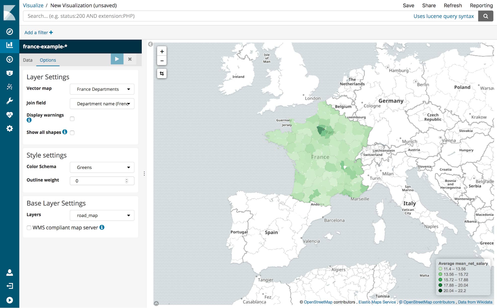
It appears that the departments around Paris have a higher mean net salary. That’s probably not a big surprise though. Let’s try another visualization.
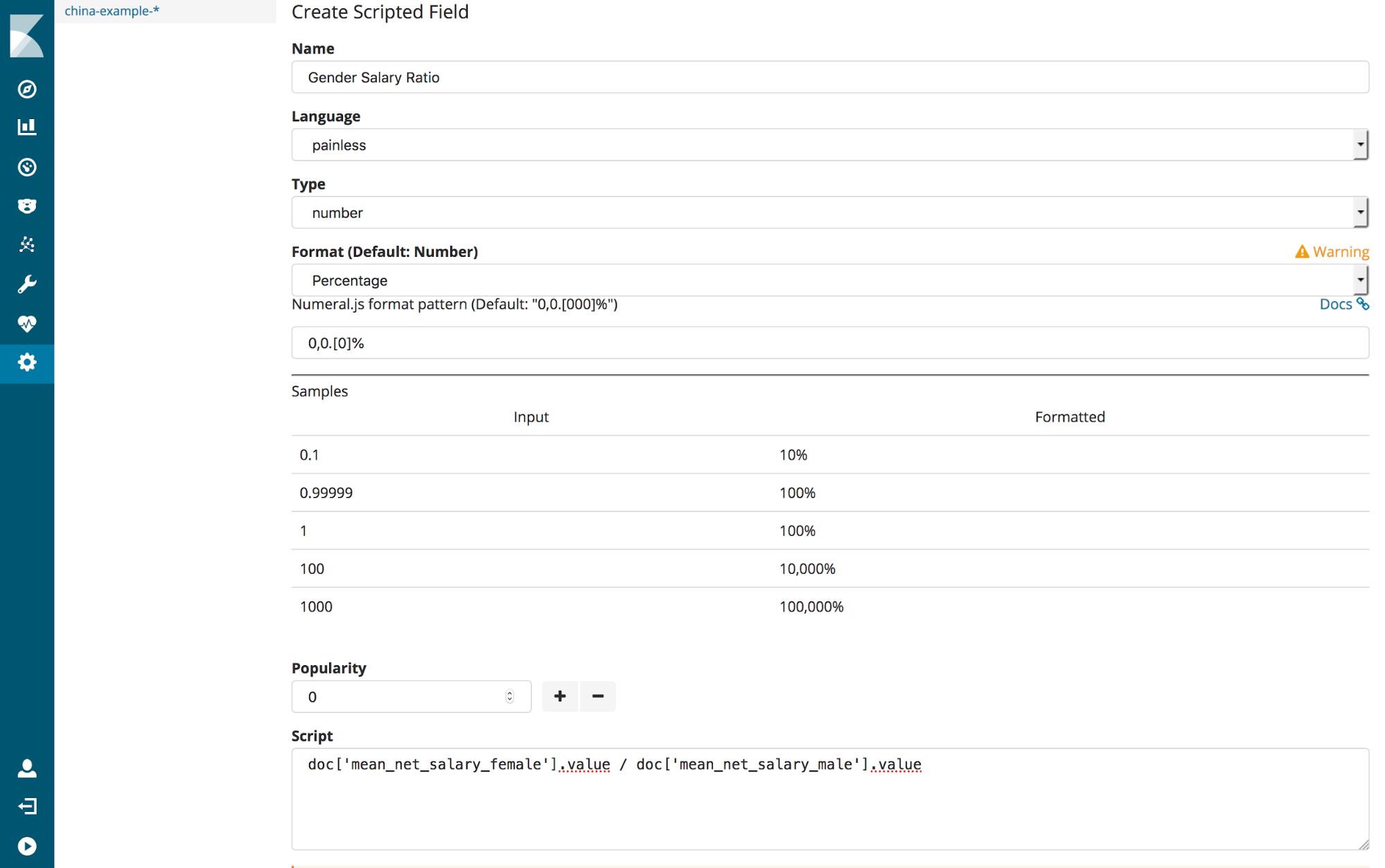
Our data has mean net salaries for males and females. So we can check for a gender pay gap for each department. To do this, we’ll need to first create a scripted field. Open the Management tab on the sidebar, select “Index Patterns” and choose the france-example-* pattern if necessary.
Open the scripted fields tab and click the “Add a Scripted Field” button. Set the name of the scripted field to Gender Salary Ratio and enter
doc['mean_net_salary_female'].value / doc['mean_net_salary_male'].value
as the script. This will calculate the ratio of female salary to male salary. You may also wish to change the format to percentage. Click the “Create Field” button to add this new field to the index.
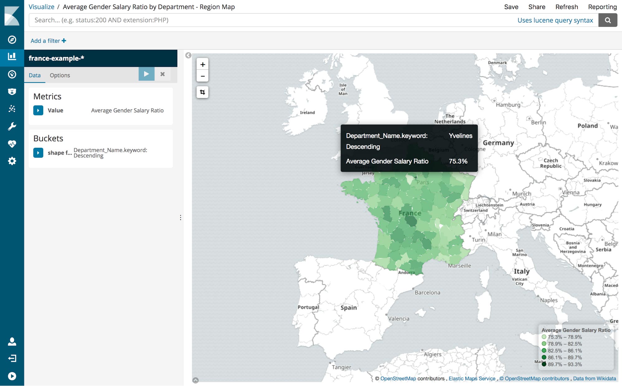
Now create a new region map visualization using the new Gender Salary Ratio field and aggregate by department name. Now we can see which departments appear to have towns with higher and lower disparities between male and female salaries.
You can explore further by creating other scripted fields for different position levels and age ranges.
Region map visualizations are available on Kibana version 5.5 and up. We are working to release more administrative regions soon. Please create an issue on the Kibana GitHub repository if there’s a region dataset that should be included in Kibana.