Custom Elasticsearch Aggregations for Machine Learning Jobs
Editor's Note (August 3, 2021): This post uses deprecated features. Please reference the map custom regions with reverse geocoding documentation for current instructions.
Recently I had a question that came up asking how to manage a derivative aggregation in a Machine Learning job. Custom aggregations are supported as part of the Machine Learning job's data feed config, and there is documentation on how to do this. There are a few specific rules that should be followed so let's go through an example from start to finish so that you can see how it is done.
For this particular example, we'll use the following data set.
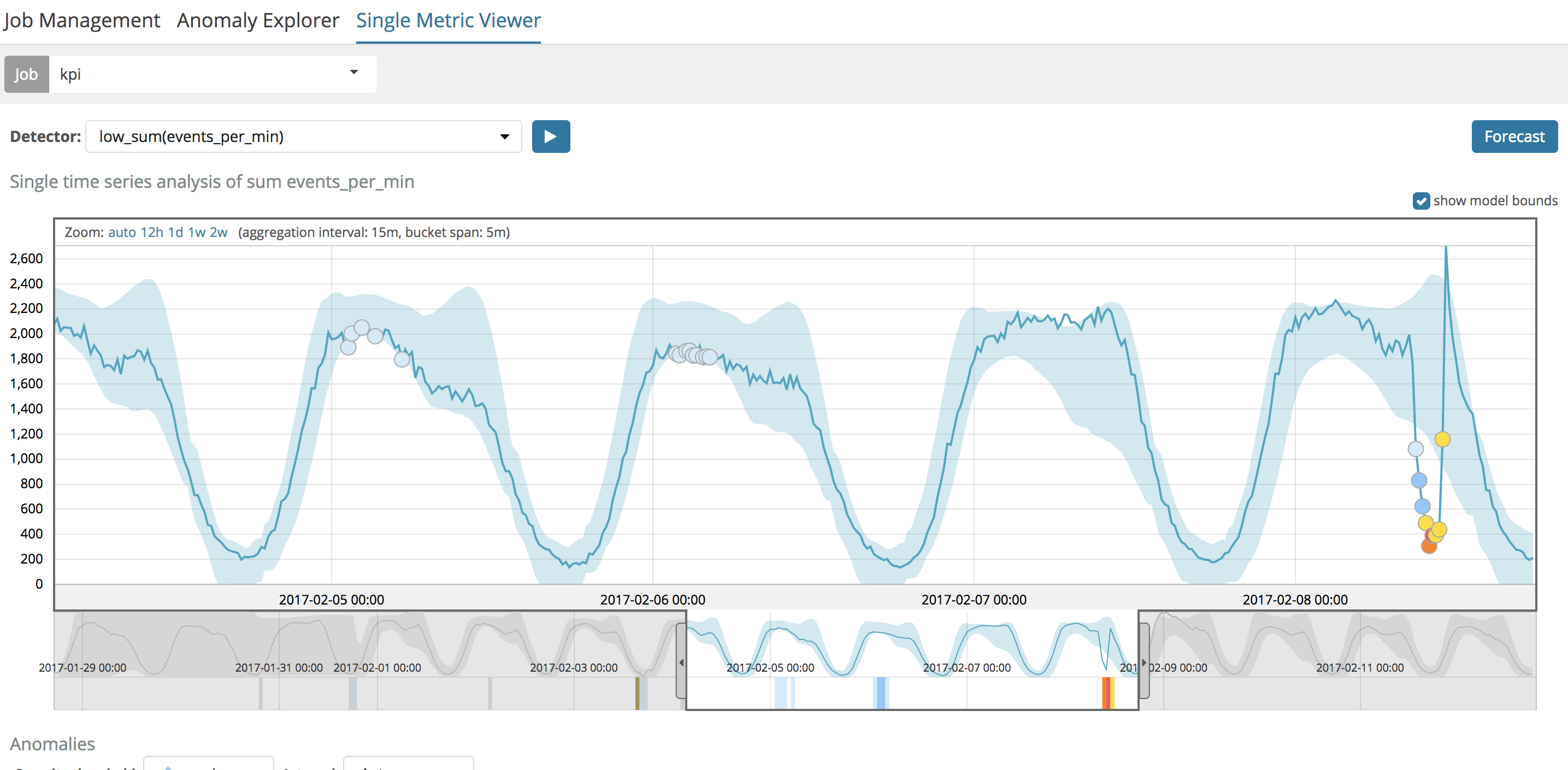
Under normal circumstances, just analyzing the data using ML's low_sum function is good enough to detect the anomaly of the "brown-out" on the last day of the data viewed above. But, for the sake of argument, let's imagine that what we're really interested is in the rate of change (the derivative) of the data set. In other words, the "recovery" coming out of the brown-out is a sharp, positive, rate of change that should have a high derivative at that moment. So, using the derivative aggregation in an Elasticsearch query, we can calculate the instantaneous rate of change and then use ML to see if the derivative is extreme at any point in time.
Defining The Job
Let's create a job config that will do this for us. I'll use the ML API (invoked via the dev Console in Kibana) to do the creation:
PUT _xpack/ml/anomaly_detectors/orders_deriv
{
  "description": "Derivative of Order Volume",
  "analysis_config": {
    "bucket_span": "5m",
    "detectors": [
      {
        "detector_description": "sum(orders_deriv)",
        "function": "sum",
        "field_name": "orders_deriv"
      }
    ],
    "influencers": [],
    "summary_count_field_name": "doc_count"
  },
  "model_plot_config": {
    "enabled": "true"
  },
  "data_description": {
    "time_field": "@timestamp"
  }
}
Notice the usage of summary_count_field_name, this is required when using aggregated queries in Machine Learning. Also note that the field_name of "orders_deriv" in the detector doesn’t exist in the raw data, it will instead come from Elasticsearch's derivative aggregation in the datafeed’s query, outlined below.
Defining the Datafeed
Let's create the datafeed which defines the source of the data to feed to the ML job:
PUT _xpack/ml/datafeeds/datafeed-orders_deriv/
{
  "job_id": "orders_deriv",
  "indices": [
    "it_ops_kpi-2017"
  ],
  "types": [
    "doc"
  ],
  "aggregations": {
    "buckets": {
      "date_histogram": {
        "field": "@timestamp",
        "interval": "5m",
        "time_zone": "UTC"
      },
      "aggregations": {
        "@timestamp": {
          "max": {
            "field": "@timestamp"
          }
        },
        "orders": {
          "sum": {
            "field": "events_per_min"
          }
        },
        "orders_deriv": {
          "derivative": {
            "buckets_path": "orders"
          }
        }
      }
    }
  }
}
As shown in the documentation, there first must be a buckets aggregation, which in turn must contain a date histogram aggregation. This requirement ensures that the aggregated data is a time series. After that, however, we do a sum aggregation (to mimic what we were doing before with ML's low_sum function) and then a derivative aggregation on that summed value. When all is said and done, Elasticsearch is creating and returning a "new" field called "orders_deriv" to the ML job.
One can test the datafeed's query and see if the outcome is as expected - just use the _preview endpoint:
GET _xpack/ml/datafeeds/datafeed-orders_deriv/_preview
The return may look something like:
[
  {
    "@timestamp": 1485643149000,
    "doc_count": 4
  },
  {
    "@timestamp": 1485643449000,
    "orders_deriv": 66,
    "doc_count": 5
  },
  {
    "@timestamp": 1485643749000,
    "orders_deriv": 20,
    "doc_count": 5
  },
  {
    "@timestamp": 1485644049000,
    "orders_deriv": -3,
    "doc_count": 5
  },
  {
    "@timestamp": 1485644349000,
    "orders_deriv": -42,
    "doc_count": 5
  },
...
The Outcome
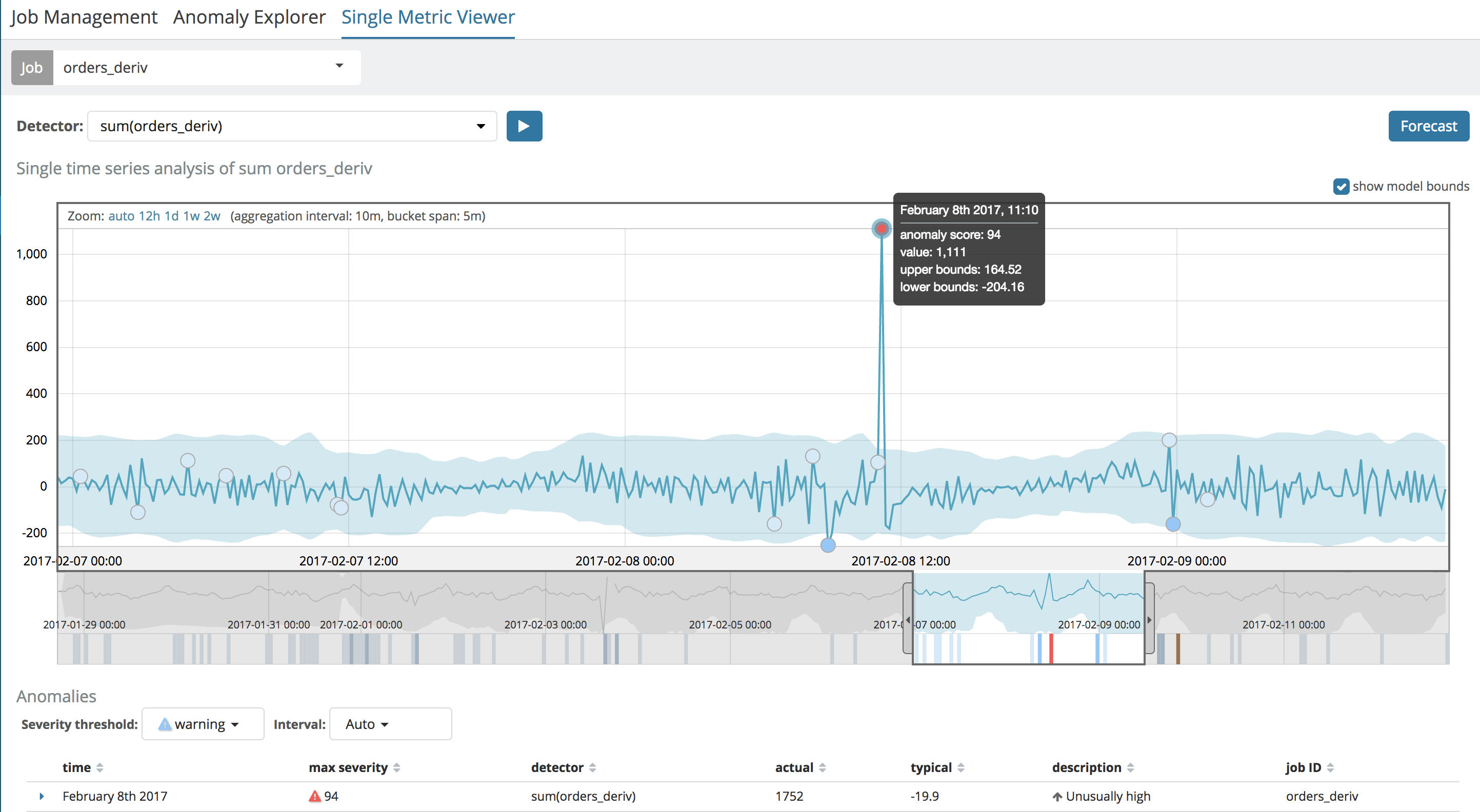
The result of running the job (either via the UI or the API) indeed shows the large, positive, rate of change at 11:10AM:
We can also "overlay" this job with a straight-up analysis of the raw data and see them together and confirm that the high derivative is when the orders sharply recover after the brown-out:
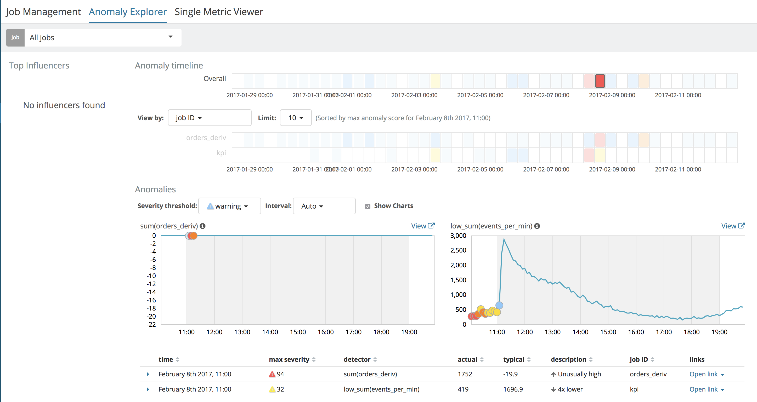
However, notice in this case, the little thumbnail graph on the left (for the derivative analysis) does not show the plot of the derivative over time like the Single Metric View does. Why is that, you might ask?
Well, it is because in the Single Metric View, the chart drawn shows the user the "actual" values from the ML model if model_plot_config is enabled. If model_plot_config is not enabled, then the "actual" values will come from a query to ES for the raw data that is executed when the view is loaded. As such, if model_plot_config is not enabled, then the Single Metric Viewer will look the same as the thumbnail chart in the Anomaly Explorer:
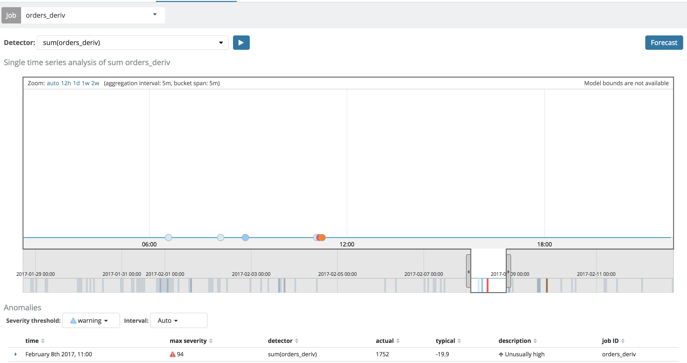
This is currently a limitation of the UI - it is unable to, on-the-fly, reverse engineer the complex Elasticsearch query that was used as part of the datafeed in order to query the raw data to draw the line. We hope to be able to support this in the future though.
You can find more about X-Pack and Machine Learning here. If you are already using Machine Learning then make sure you check out our prebuilt recipes to help bootstrap your efforts.