Implementing a statistical anomaly detector in Elasticsearch - Part 2
Last week, we built a pipeline aggregation which distills thousands of data-points into a handful of representative metrics. This forms the basis of Atlas, and does all the heavy lifting required to implement the anomaly detector. This week, we'll finish the implementation and generate some fun graphs.
The aggregation we built is designed to be run over a specific window of time: given a date range, it will emit a 90th percentile surprise value for each metric. To fully implement Atlas, we need to plot those 90th percentile values themselves over time. This functionality is not currently possible using just Pipeline aggs (although a "sliding histogram" functionality has been proposed which would fill the gap).
Instead, we are going to move the responsibility to TimeLion, which is well suited for this type of post-processing (Timelion is a new {Re}search project to put fluent time-series manipulation inside Kibana; you can read more about it here).
If you revisit the simulator code, you'll see that we run a series of queries after the data has been generated. We slide our Pipeline agg across the data in one-hour increments (with a window size of 24 hours). We also use filter_path to minimize the response output: we don't actually care about the 60,000 buckets… we just want the "ninetieth_surprise" from each metric. Filtering the response cuts down network transfer considerably. The values are then indexed back into Elasticsearch so we can chart them later.
We pre-processed these values ahead of time in the simulator to simplify the demonstration, but in a real system you'd likely have a Watcher or cronjob executing the query every hour and saving the results.
Plotting 90th percentile surprise
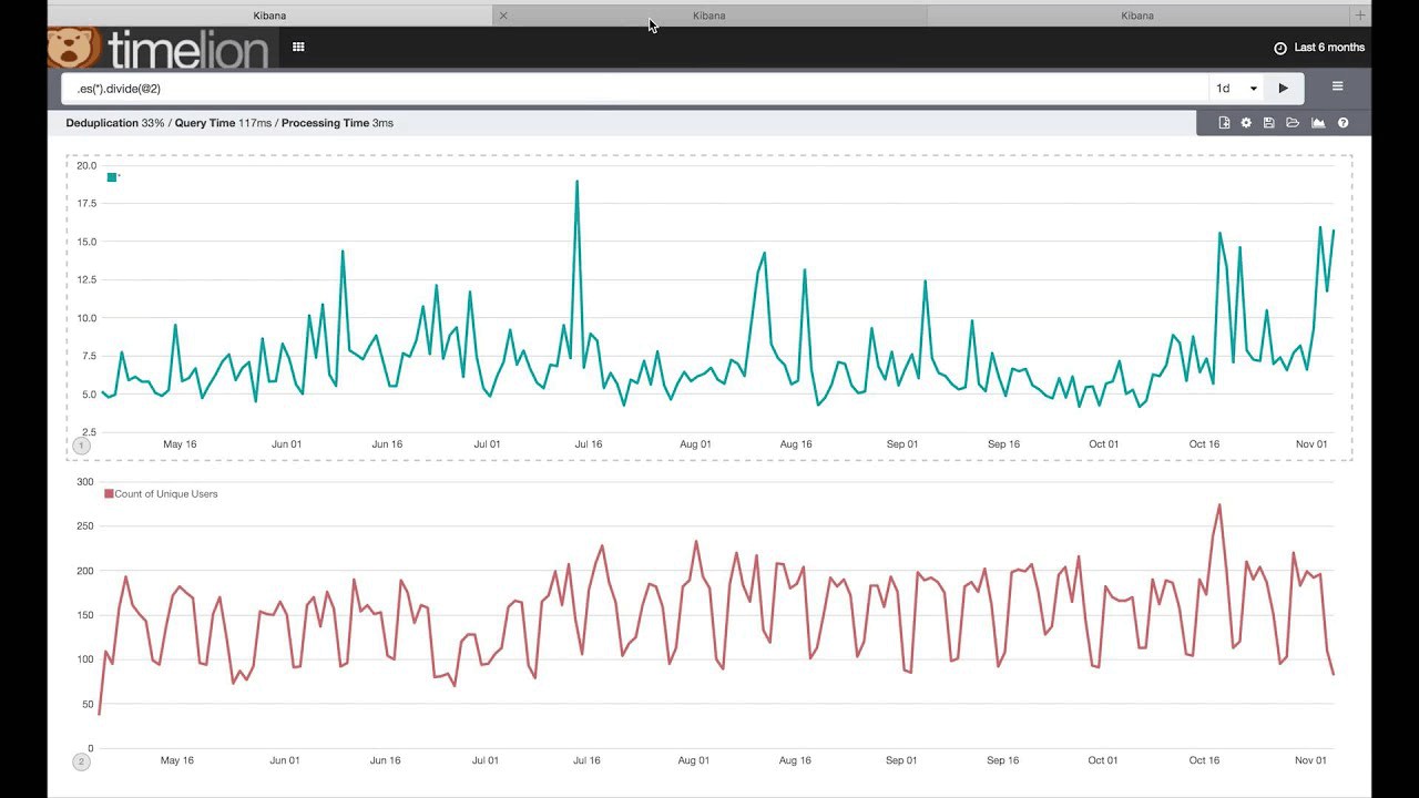
With the heavy lifting done last week, we can turn to TimeLion to finish the implementation. The first order of business is to pull down the 90th values for a particular metric. We can do that with the following TimeLion syntax:
.es('metric:0', metric='avg:value').label("#0 90th surprise")
Which will generate a graph that looks something like this:
Well that looks fun! There is definitely something happening. Let's walk through what this chart means, since it is fundamental to how Atlas works:
- Last week, we calculated the "surprise" of each time-series: the deviation from it's own moving average
- We then collected the top 90th percentile of these "surprise" values, and are now plotting them over time
- Effectively, this chart is showing us the variability of the top "surprise" (deviations).
- A large spike in this chart means the data has become more surprising ... the top 90th percentiles has changed drastically (up or down, since we used an absolute value to calculate surprise)
Effectively, if we see a spike we can conclude the underlying data has changed enough to shift our normal variance, likely due to a disruption. This is the heart of Atlas: don't watch your data because there is just too much. Instead, watch the variance of the 90th percentile of deviations from the mean.
If you compare the above graph to the actual data for metric #0, you’ll see the stark difference:
Building the Atlas Dashboard
Of course, the trick is to now automatically identify those spikes and graph/alert on them. Let's start building that logic. Atlas alerts when the 90th percentile surprise is 3 standard deviations above the moving average. If you decompose that problem, you'll see several necessary components:
- A rolling, three standard deviation
- A rolling average of the data
- Adding the rolling std on top of the rolling data. This represents the "threshold" the data must stay below
- Alerting when the data breaches the "threshold"
First, we construct the rolling three standard deviations. We do this with a custom movingstd() function (see footnote for source, it is essentially identical to a movingavg() function), then multiply it by three to get the third sigma:
Note: I'm indenting all the queries to make them easier to read
.es('metric:0', metric='avg:value')
 .movingstd(6)
 .multiply(3)
Next we write a snippet to calculate a rolling average of the data itself:
.es('metric:0', metric='avg:value')
 .movingaverage(6)
And finally, we combine those two snippets by adding them together to create the "threshold". This will create a line that is three standard deviations above the moving average of the data:
.es('metric:0', metric='avg:value')
  .movingaverage(6)
  .sum(
    .es('metric:0', metric='avg:value')
      .movingstd(6)
      .multiply(3)
  )
Now that we have a "threshold", we can plot this with the original data and see how they compare:
Hmm, ok. It's not really clear right now if the threshold is working or not. The chart is difficult to read; as soon as the surprise value spikes it causes a subsequent spike in the threshold. This happens because the spike causes a large change in variance, which the rolling stddev picks up, causing the threshold itself to shoot up.
If we zoom in on the first spike, we can see that the 90th percentile briefly passes the threshold before the rolling stddev "catches up":
(Apologies, this chart is mislabeled: "metric: 0" should read "#0 Threshold")
It's now clear: we want to show is the moment in time when the surprise crosses the threshold, and ignore the threshold otherwise (since it is only useful in that first instant). Let’s display a single bar when it crosses the threshold instead of a continuous line.
To do that, we add a custom showifgreater() function. This will only show data-points in the first series if they are greater than the data-points in the second series (see footnote for source):
.es('metric:0', metric='avg:value').showifgreater(...)
And to complete our query, we only want to show the data if it is greater than three standard deviations (aka if it breaches than the threshold), and then we want to show it as bars instead of lines. That gives us our final query:
.es('metric:0', metric='avg:value')
 .showifgreater(
   .es('metric:0', metric='avg:value')
    .movingaverage(6)
    .sum(
      .es('metric:0', metric='avg:value')
      .movingstd(6)
      .multiply(3)
    )
  ).bars()
  .yaxis(2)
  .label("#0 anomalies")
Which generates a much nicer looking chart:
Finally, let's add back the data itself so we have something to compare against:
.es('metric:0', metric='avg:value')
 .label("#0 90th surprise"),
.es('metric:0', metric='avg:value')
 .showifgreater(
   .es('metric:0', metric='avg:value')
    .movingaverage(6)
    .sum(
      .es('metric:0', metric='avg:value')
      .movingstd(6)
      .multiply(3)
    )
  ).bars()
  .yaxis(2)
  .label("#0 anomalies")
Voila! We've implemented Atlas! The complete dashboard includes a chart for each metric, as well as a chart showing when disruptions were created (which you obviously would not have in a production environment, but is useful for verifying our simulation):
Analysis of anomalies
If you work through the disruption chart (top-left), you'll find an associated anomaly in at least one of the metric charts, often in several simultaneously. Encouragingly, anomalies are tagged for all types of disruptions (node, query, metric). The footnote contains a list of the disruptions and their magnitude to give you an idea of impact. For example, one "Query Disruption" lasted three hours and only affected 12 of the 500 total queries (2.4%)
One phenomenon you see in the charts are spikes that stay elevated for a while. This is in part due to the duration of the disruption, some which last multiple hours. But it is also due to the limitation in our pipeline agg mentioned last week: namely, we are selecting the "largest" surprise from each timeseries, not the "last" surprise. That means disruptions are drawn out for an extra 24 hours in the worst case, because the surprise only resets once the disruption falls out of the window. This is entirely dependent on the chosen window sizes, and the sensitivity can be tuned by increasing/decreasing the window.
This phenomenon doesn't affect anomaly detection much, although it becomes more apparent if you try to use longer windows of time. Once pipeline aggs have the ability to select "last", this should be resolved.
Conclusion
So, that's Atlas. A fairly simple -- but very effective -- statistical anomaly detection system built at eBay, and now implemented in Elasticsearch + Timelion. Prior to Pipeline aggs, this could have been implemented by a lot of client-side logic. But the prospect of streaming 60k buckets back to the client every hour for processing is not enticing... pipeline aggs have moved the heavy lifting to the server for more efficient processing.
Pipeline aggs are still very young, so expect more functionality to be added over time. If you have a use-case that is difficult to express in pipelines, please let us know!
The end! Or is it...
"But wait!" you say, "this is just plotting the anomalies. How do I get alerts?" For that answer, you'll have to wait until next week, when we implement the TimeLion syntax as a Watcher watch so that you can get automated alerts to email, Slack, etc. See you next week!
Footnotes
- The custom
movingstd()andshowifgreater()Timelion functions can be found here. Shut down Kibana, add the functions to your Timelion source (kibana/installedPlugins/timelion/series_functions/<function_name>.js), delete the optimized bundle (rm kibana/optimize/bundles/timelion.bundle.js) and restart Kibana. The functions should be available for use in Timelion now. Note: Javascript is not my forte, so these are not elegant examples of code :) - The disruptions that were simulated are attached below. The format is in the format: Disruption type: hour_start-hour_end [affected nodes/queries/metrics]
- Metric Disruption: 505-521 [0, 3, 4]
- Metric Disruption: 145-151 [3, 4]
- Node Disruption: 279-298 [0]
- Metric Disruption: 240-243 [1]
- Query Disruption: 352-355 [5, 23, 27, 51, 56, 64, 65, 70, 72, 83, 86, 95, 97, 116, 135, 139, 181, 185, 195, 200, 206, 231, 240, 263, 274, 291, 295, 307, 311, 315, 322, 328, 337, 347, 355, 375, 385, 426, 468]
- Metric Disruption: 172-181 [0, 2]
- Node Disruption: 334-337 [0]
- Query Disruption: 272-275 [63, 64, 168, 179, 193, 204, 230, 295, 308, 343, 395, 458]
- After last week's article, there were some questions regarding the nature of the data: namely, the data was generated using normal (gaussian) curves. Would Atlas work with skewed data, since much data in real life doesn't follow a nice normal distribution? I ran a quick test using LogNormal curves which skew heavily to the left, and it appear Atlas continues to function well. The Atlas paper corroborates this empirical evidence. Atlas relies on the 90th surprise over time to be somewhat normal, which seems to hold true even if the underlying data is heavily skewed. There may be followup articles about Atlas behavior under different data distributions as I find time to experiment.