WARNING: Version 5.5 of the Elastic Stack has passed its EOL date.
This documentation is no longer being maintained and may be removed. If you are running this version, we strongly advise you to upgrade. For the latest information, see the current release documentation.
Creating Single Metric Jobs
editCreating Single Metric Jobs
editMachine learning jobs contain the configuration information and metadata necessary to perform an analytical task. They also contain the results of the analytical task.
This tutorial uses Kibana to create jobs and view results, but you can alternatively use APIs to accomplish most tasks. For API reference information, see Machine Learning APIs.
The X-Pack machine learning features in Kibana use pop-ups. You must configure your web browser so that it does not block pop-up windows or create an exception for your Kibana URL.
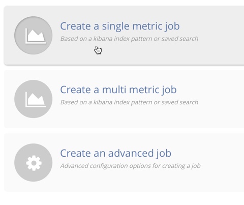
You can choose to create single metric, multi-metric, or advanced jobs in Kibana. At this point in the tutorial, the goal is to detect anomalies in the total requests received by your applications and services. The sample data contains a single key performance indicator to track this, which is the total requests over time. It is therefore logical to start by creating a single metric job for this KPI.
If you are using aggregated data, you can create an advanced job
and configure it to use a summary_count_field_name. The machine learning algorithms will
make the best possible use of summarized data in this case. For simplicity, in
this tutorial we will not make use of that advanced functionality.
A single metric job contains a single detector. A detector defines the type of
analysis that will occur (for example, max, average, or rare analytical
functions) and the fields that will be analyzed.
To create a single metric job in Kibana:
-
Open Kibana in your web browser. If you are running Kibana locally,
go to
http://localhost:5601/. -
Click Machine Learning in the side navigation:
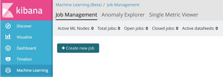
- Click Create new job.
-
Click Create single metric job.
-
Click the
server-metricsindex.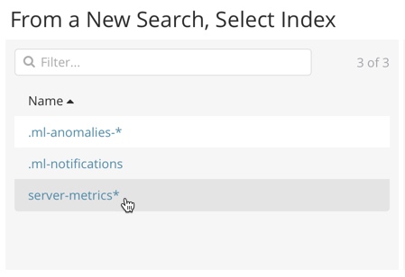
-
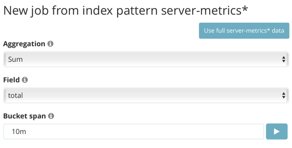
Configure the job by providing the following information:
-
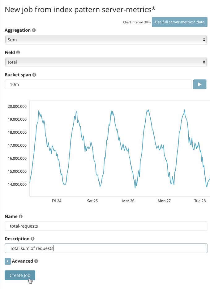
For the Aggregation, select
Sum. This value specifies the analysis function that is used.Some of the analytical functions look for single anomalous data points. For example,
maxidentifies the maximum value that is seen within a bucket. Others perform some aggregation over the length of the bucket. For example,meancalculates the mean of all the data points seen within the bucket. Similarly,countcalculates the total number of data points within the bucket. In this tutorial, you are using thesumfunction, which calculates the sum of the specified field’s values within the bucket. -
For the Field, select
total. This value specifies the field that the detector uses in the function.Some functions such as
countandraredo not require fields. -
For the Bucket span, enter
10m. This value specifies the size of the interval that the analysis is aggregated into.The X-Pack machine learning features use the concept of a bucket to divide up the time series into batches for processing. For example, if you are monitoring the total number of requests in the system, using a bucket span of 1 hour would mean that at the end of each hour, it calculates the sum of the requests for the last hour and computes the anomalousness of that value compared to previous hours.
The bucket span has two purposes: it dictates over what time span to look for anomalous features in data, and also determines how quickly anomalies can be detected. Choosing a shorter bucket span enables anomalies to be detected more quickly. However, there is a risk of being too sensitive to natural variations or noise in the input data. Choosing too long a bucket span can mean that interesting anomalies are averaged away. There is also the possibility that the aggregation might smooth out some anomalies based on when the bucket starts in time.
The bucket span has a significant impact on the analysis. When you’re trying to determine what value to use, take into account the granularity at which you want to perform the analysis, the frequency of the input data, the duration of typical anomalies and the frequency at which alerting is required.
-
-
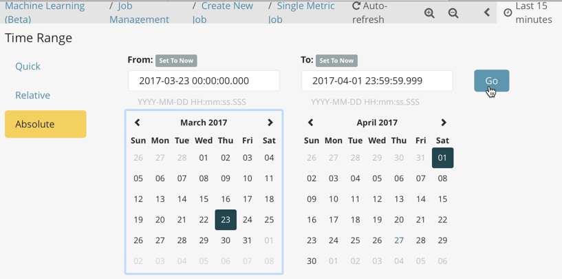
Determine whether you want to process all of the data or only part of it. If you want to analyze all of the existing data, click Use full server-metrics* data. If you want to see what happens when you stop and start datafeeds and process additional data over time, click the time picker in the Kibana toolbar. Since the sample data spans a period of time between March 23, 2017 and April 22, 2017, click Absolute. Set the start time to March 23, 2017 and the end time to April 1, 2017, for example. Once you’ve got the time range set up, click the Go button.
A graph is generated, which represents the total number of requests over time.
-
Provide a name for the job, for example
total-requests. The job name must be unique in your cluster. You can also optionally provide a description of the job. -
Click Create Job.
As the job is created, the graph is updated to give a visual representation of the progress of machine learning as the data is processed. This view is only available whilst the job is running.
The create_single_metric.sh script creates a similar job and datafeed by
using the machine learning APIs. Before you run it, you must edit the USERNAME and PASSWORD
variables with your actual user ID and password. If X-Pack security is not enabled,
use the create_single_metric_noauth.sh script instead. For API reference
information, see Machine Learning APIs.