Predicting delayed flights with classification analysis
editPredicting delayed flights with classification analysis
editLet’s try to predict whether a flight will be delayed or not by using the sample flight data. We want to be able to use information such as weather conditions, carrier, flight distance, origin, or destination to predict flight delays. There are only two possible outcome values: the flight is either delayed or not, therefore we use binary classification to make the prediction.
We have chosen this data set as an example because it is easily accessible for Kibana users and the use case is relevant. However, the data has been manually created and contains some inconsistencies. For example, a flight can be both delayed and canceled. Please remember that the quality of your input data affects the quality of your results.
Each document in the data set contains details for a single flight, so this data is ready for analysis; it is already in a two-dimensional entity-based data structure (data frame). In general, you often need to transform the data into an entity-centric index before you analyze the data.
Example source document
{
  "_index": "kibana_sample_data_flights",
  "_type": "_doc",
  "_id": "S-JS1W0BJ7wufFIaPAHe",
  "_version": 1,
  "_seq_no": 3356,
  "_primary_term": 1,
  "found": true,
  "_source": {
    "FlightNum": "N32FE9T",
    "DestCountry": "JP",
    "OriginWeather": "Thunder & Lightning",
    "OriginCityName": "Adelaide",
    "AvgTicketPrice": 499.08518599798685,
    "DistanceMiles": 4802.864932998549,
    "FlightDelay": false,
    "DestWeather": "Sunny",
    "Dest": "Chubu Centrair International Airport",
    "FlightDelayType": "No Delay",
    "OriginCountry": "AU",
    "dayOfWeek": 3,
    "DistanceKilometers": 7729.461862731618,
    "timestamp": "2019-10-17T11:12:29",
    "DestLocation": {
      "lat": "34.85839844",
      "lon": "136.8049927"
    },
    "DestAirportID": "NGO",
    "Carrier": "ES-Air",
    "Cancelled": false,
    "FlightTimeMin": 454.6742272195069,
    "Origin": "Adelaide International Airport",
    "OriginLocation": {
      "lat": "-34.945",
      "lon": "138.531006"
    },
    "DestRegion": "SE-BD",
    "OriginAirportID": "ADL",
    "OriginRegion": "SE-BD",
    "DestCityName": "Tokoname",
    "FlightTimeHour": 7.577903786991782,
    "FlightDelayMin": 0
  }
}
Each document in this sample data contains a FlightDelay field with a boolean
value. Classification is a supervised machine learning analysis and therefore
needs to train on data that contains the ground truth, known as the
dependent_variable. In this example, the ground truth is available in each
document as the actual value of FlightDelay. In order to be analyzed, a
document must contain at least one field with a supported data type (numeric,
boolean, text, keyword or ip) and must not contain arrays with more than
one item.
If your source data consists of some documents that contain a dependent variable and some that do not, the model is trained on the subset of documents that contain ground truth. By default, all of that subset of documents is used for training. However, you can choose to specify a percentage of the documents as your training data. Predictions are made against all of the data. The current implementation of classification analysis supports a single batch analysis for both training and predictions.
Creating a classification model
editTo predict whether a specific flight is delayed:
-
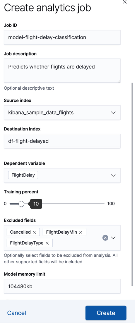
Create a data frame analytics job.
You can use the wizard on the Machine Learning > Data Frame Analaytics tab in Kibana or the create data frame analytics jobs API.
-
Choose
classificationas the job type. -
Choose
kibana_sample_data_flightsas the source index. - Add the name of the destination index that will contain the results of the analysis. It will contain a copy of the source index data where each document is annotated with the results. If the index does not exist, it will be created automatically.
-
Choose
FlightDelayas the dependent variable, which is the field that we want to predict with the classification analysis. -
Choose a training percent of
10which means it randomly selects 10% of the source data for training. While that value is low for this example, for many large data sets using a small training sample greatly reduces runtime without impacting accuracy. -
Add
Cancelled,FlightDelayMin, andFlightDelayTypeto the list of excluded fields. These fields will be excluded from the analysis. It is recommended to exclude fields that either contain erroneous data or describe thedependent_variable. - Use the default memory limit for the job. If the job requires more than this amount of memory, it fails to start. If the available memory on the node is limited, this setting makes it possible to prevent job execution.
API example
PUT _ml/data_frame/analytics/model-flight-delay-classification { "source": { "index": [ "kibana_sample_data_flights" ] }, "dest": { "index": "df-flight-delayed", "results_field": "ml" }, "analysis": { "classification": { "dependent_variable": "FlightDelay", "training_percent": 10 } }, "analyzed_fields": { "includes": [], "excludes": [ "Cancelled", "FlightDelayMin", "FlightDelayType" ] }, "model_memory_limit": "100mb" } -
Choose
-
Start the job in Kibana or use the start data frame analytics jobs API.
The job takes a few minutes to run. Runtime depends on the local hardware and also on the number of documents and fields that are analyzed. The more fields and documents, the longer the job runs. It stops automatically when the analysis is complete.
API example
POST _ml/data_frame/analytics/model-flight-delay-classification/_start
-
Check the job stats to follow the progress in Kibana or use the get data frame analytics jobs statistics API.
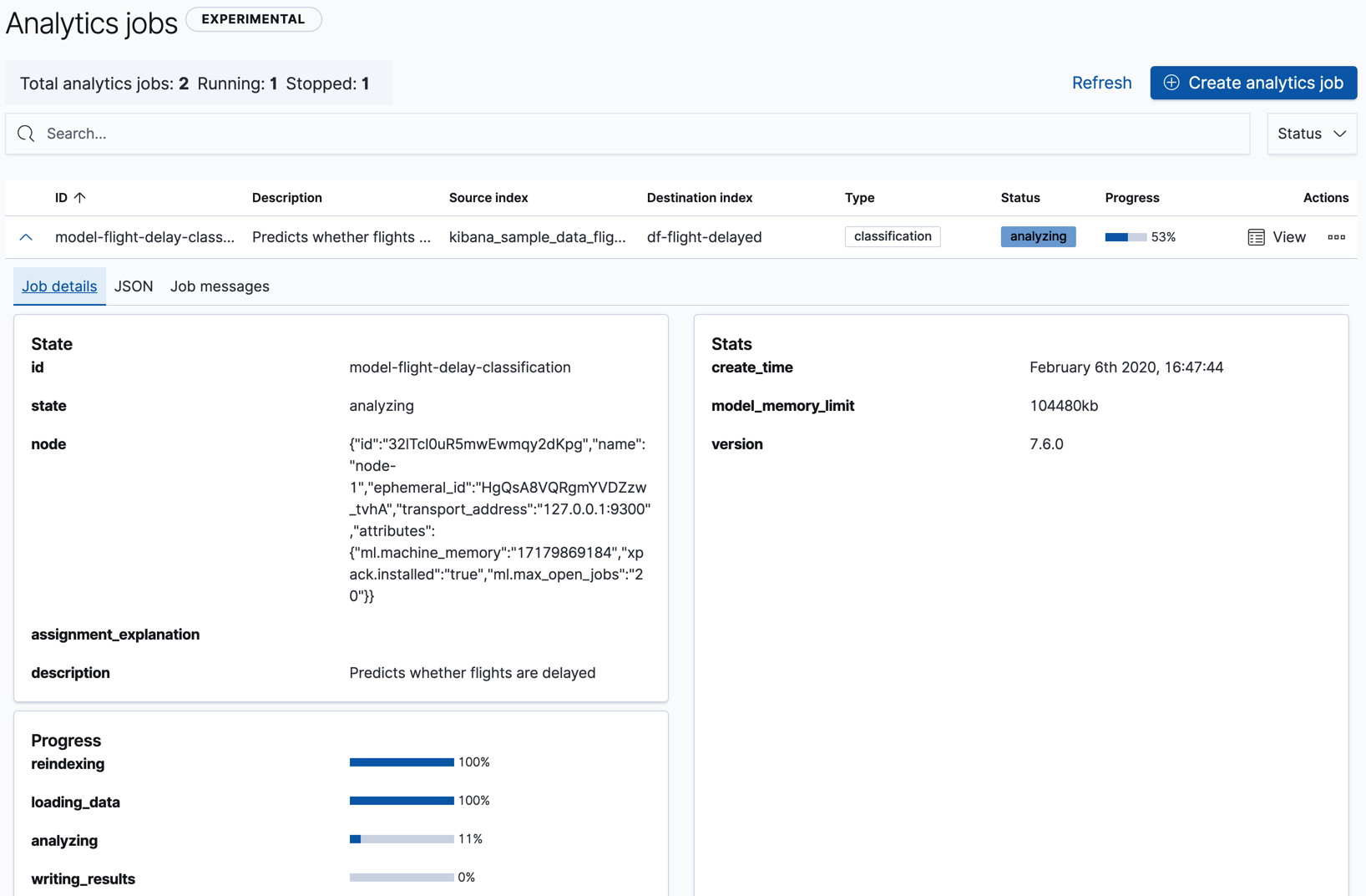
The job has four phases (reindexing, loading data, analyzing, and writing results). When all the phases have completed, the job stops and the results are ready to view and evaluate.
API example
GET _ml/data_frame/analytics/model-flight-delay-classification/_stats
The API call returns the following response:
{
  "count" : 1,
  "data_frame_analytics" : [
    {
      "id" : "model-flight-delay-classification",
      "state" : "stopped",
      "progress" : [
        {
          "phase" : "reindexing",
          "progress_percent" : 100
        },
        {
          "phase" : "loading_data",
          "progress_percent" : 100
        },
        {
          "phase" : "analyzing",
          "progress_percent" : 100
        },
        {
          "phase" : "writing_results",
          "progress_percent" : 100
        }
      ]
    }
  ]
}
Viewing classification results
editNow you have a new index that contains a copy of your source data with predictions for your dependent variable.
When you view the classification results in Kibana, it shows contents of the destination index in a tabular format:
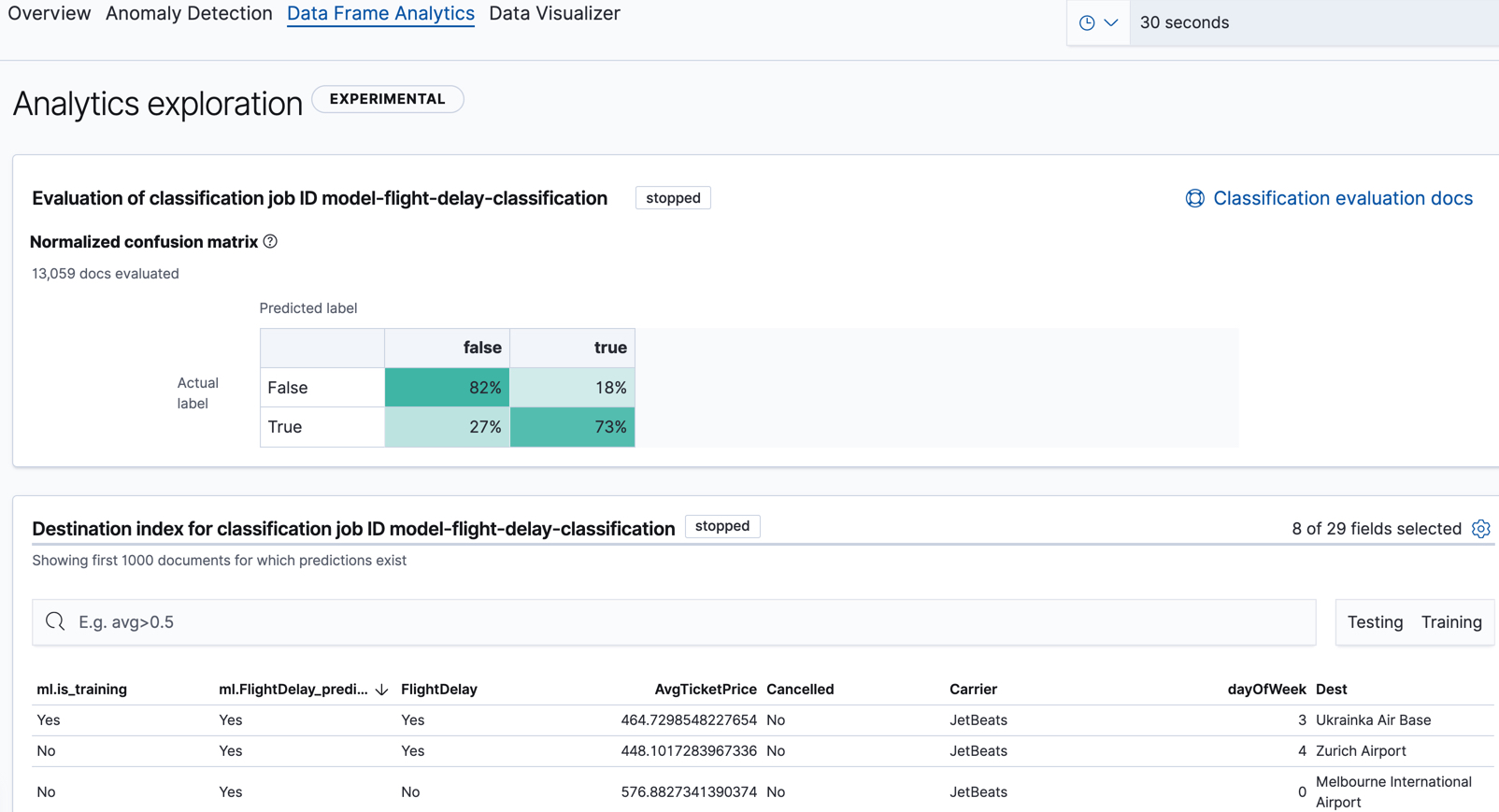
In this example, the table shows a column for the dependent variable
(FlightDelay), which contains the ground truth values that we are trying to
predict with the classification analysis. It also shows a column for the prediction values
(ml.FlightDelay_prediction) and a column that indicates whether the
document was used in the training set (ml.is_training). You can filter the
table to show only testing or training data and you can change which fields are
shown in the table.
If you examine this destination index more closely in the Discover app in Kibana
or use the standard Elasticsearch search command, you can see that the analysis predicts
the probability of all possible classes for the dependent variable (in a
top_classes object). In this case, there are two classes: true and false.
The most probable class is the prediction, which is what’s shown in the
classification results table. If you want to understand how sure the model is
about the prediction, however, you might want to examine the class probability
values. A higher number means that the model is more confident.
API example
GET df-flight-delayed/_search
The snippet below shows a part of a document with the annotated results:
          ...
          "FlightDelay" : false,
          ...
          "ml" : {
            "top_classes" : [
              {
                "class_probability" : 0.939335365058496,
                "class_score" : 0.6757432490367542,
                "class_name" : "false"
              },
              {
                "class_probability" : 0.06066463494150393,
                "class_score" : 0.06835090015710144,
                "class_name" : "true"
              }
            ],
            "FlightDelay_prediction" : "false",
            "is_training" : false
          }
|
An array of values specifying the probability of the prediction and the
|
|
|
The probability is a value between 0 and 1. The higher the number, the more
confident the model is that the data point belongs to the named class. In this
example, |
|
|
The |
Evaluating classification results
editThough you can look at individual results and compare the predicted value
(ml.FlightDelay_prediction) to the actual value (FlightDelay), you
typically need to evaluate the success of your classification model as a
whole.
Kibana provides a normalized confusion matrix that contains the percentage of occurrences where the analysis classified data points correctly with their actual class and the percentage of occurrences where it misclassified them.
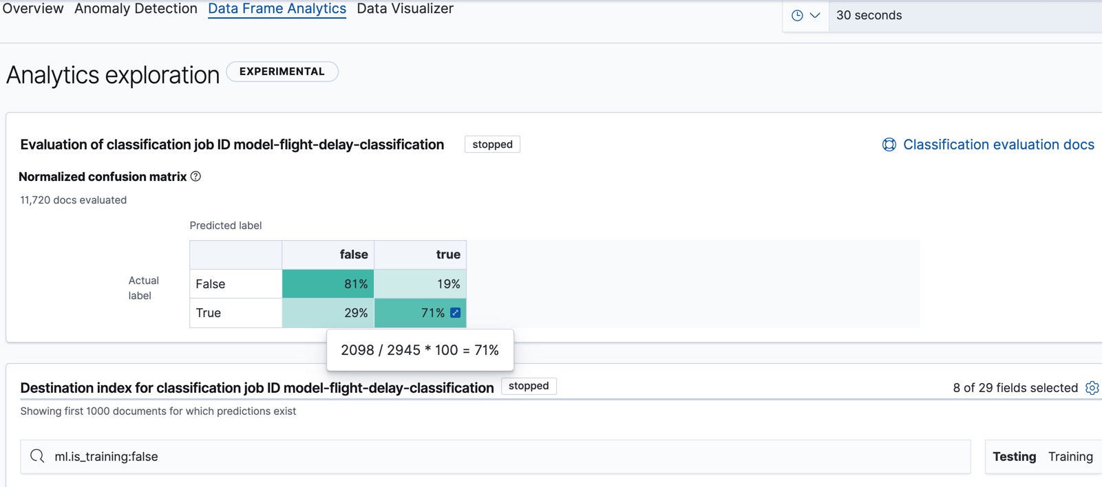
If you want to see the exact number of occurrences, select a quadrant in the
matrix. In this example, we’ve filtered the table to contain only testing data
so we can see how well the model performs on previously unseen data. There are
2945 documents in the testing data that have the true class. 847 of them are
predicted as false; this is called a false negative. 2098 are predicted
correctly as true; this is called a true positive. The confusion matrix
therefore shows us that 71% of the actual true values were correctly predicted
and 29% were incorrectly predicted in the test data set.
Likewise if you select other quadrants in the matrix, it shows you that there
are 8775 documents that have the false class as their actual value in the
testing data set. The model labeled 7093 documents (out of 8775) correctly as
false; this is called a true negative. 1682 documents are predicted
incorrectly as true; this is called a false positive. Thus 81% of the actual
false values were correctly predicted and 19% were incorrectly predicted in
the test data set.
For more information about interpreting the evaluation metrics, see Classification evaluation.
You can also generate these metrics with the data frame analytics evaluate API.
API example
First, we want to know the training error that represents how well the model performed on the training data set.
POST _ml/data_frame/_evaluate
{
 "index": "df-flight-delayed",
   "query": {
    "term": {
      "ml.is_training": {
        "value": true
      }
    }
  },
 "evaluation": {
   "classification": {
     "actual_field": "FlightDelay",
     "predicted_field": "ml.FlightDelay_prediction",
     "metrics": {
       "multiclass_confusion_matrix" : {}
     }
   }
 }
}
Next, we calculate the generalization error that represents how well the model performed on previously unseen data:
POST _ml/data_frame/_evaluate
{
 "index": "df-flight-delayed",
   "query": {
    "term": {
      "ml.is_training": {
        "value": false
      }
    }
  },
 "evaluation": {
   "classification": {
     "actual_field": "FlightDelay",
     "predicted_field": "ml.FlightDelay_prediction",
     "metrics": {
       "multiclass_confusion_matrix" : {}
     }
   }
 }
}
The returned confusion matrix shows us how many data points were classified
correctly (where the actual_class matches the predicted_class) and how many
were misclassified (actual_class does not match predicted_class):
{
  "classification" : {
    "multiclass_confusion_matrix" : {
      "confusion_matrix" : [
        {
          "actual_class" : "false",
          "actual_class_doc_count" : 8775,
          "predicted_classes" : [
            {
              "predicted_class" : "false",
              "count" : 7093
            },
            {
              "predicted_class" : "true",
              "count" : 1682
            }
          ],
          "other_predicted_class_doc_count" : 0
        },
        {
          "actual_class" : "true",
          "actual_class_doc_count" : 2945,
          "predicted_classes" : [
            {
              "predicted_class" : "false",
              "count" : 847
            },
            {
              "predicted_class" : "true",
              "count" : 2098
            }
          ],
          "other_predicted_class_doc_count" : 0
        }
      ],
      "other_actual_class_count" : 0
    }
  }
}
As the sample data may change when it is loaded into Kibana, the results of the classification analysis can vary even if you use the same configuration as the example.
If you don’t want to keep the data frame analytics job, you can delete it by using the delete data frame analytics job API. When you delete data frame analytics jobs, the destination indices remain intact.