Creating Multi-metric Jobs
editCreating Multi-metric Jobs
editThe multi-metric job wizard in Kibana provides a simple way to create more complex jobs with multiple detectors. For example, in the single metric job, you were tracking total requests versus time. You might also want to track other metrics like average response time or the maximum number of denied requests. Instead of creating jobs for each of those metrics, you can combine them in a multi-metric job.
You can also use multi-metric jobs to split a single time series into multiple time series based on a categorical field. For example, you can split the data based on its hostnames, locations, or users. Each time series is modeled independently. By looking at temporal patterns on a per entity basis, you might spot things that might have otherwise been hidden in the lumped view.
Conceptually, you can think of this as running many independent single metric jobs. By bundling them together in a multi-metric job, however, you can see an overall score and shared influencers for all the metrics and all the entities in the job. Multi-metric jobs therefore scale better than having many independent single metric jobs and provide better results when you have influencers that are shared across the detectors.
The sample data for this tutorial contains information about the requests that are received by various applications and services in a system. Let’s assume that you want to monitor the requests received and the response time. In particular, you might want to track those metrics on a per service basis to see if any services have unusual patterns.
To create a multi-metric job in Kibana:
-
Open Kibana in your web browser. If you are running Kibana locally,
go to
http://localhost:5601/. - Click Machine Learning in the side navigation, then click Create new job.
-
Select the index pattern that you created for the sample data. For example,
server-metrics*. - In the Use a wizard section, click Multi metric.
-
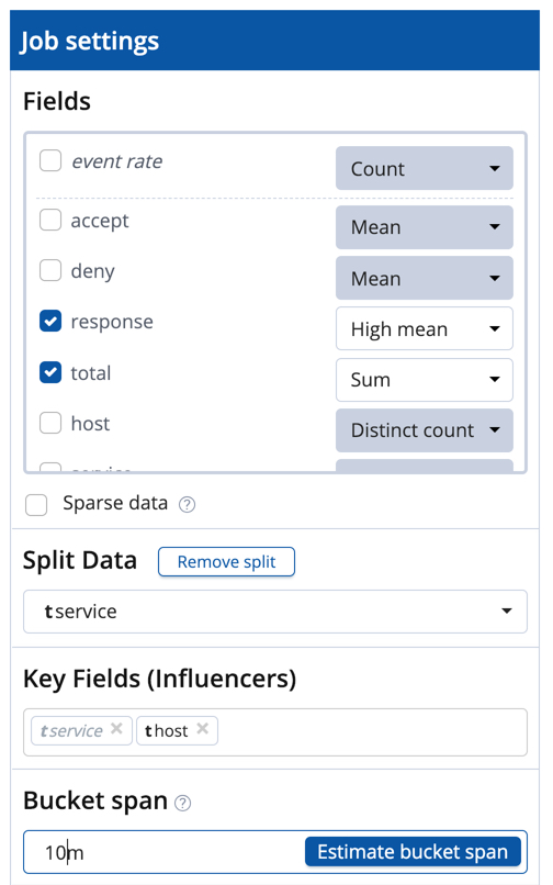
Configure the job by providing the following job settings:
-
For the Fields, select
high mean(response)andsum(total). This creates two detectors and specifies the analysis function and field that each detector uses. The first detector uses the high mean function to detect unusually high average values for theresponsefield in each bucket. The second detector uses the sum function to detect when the sum of thetotalfield is anomalous in each bucket. For more information about any of the analytical functions, see Function reference. -
For the Bucket span, enter
10m. This value specifies the size of the interval that the analysis is aggregated into. As was the case in the single metric example, this value has a significant impact on the analysis. When you’re creating jobs for your own data, you might need to experiment with different bucket spans depending on the frequency of the input data, the duration of typical anomalies, and the frequency at which alerting is required. -
For the Split Data, select
service. When you specify this option, the analysis is segmented such that you have completely independent baselines for each distinct value of this field. There are seven unique service keyword values in the sample data. Thus for each of the seven services, you will see the high mean response metrics and sum total metrics.If you are creating a job by using the machine learning APIs or the advanced job wizard in Kibana, you can accomplish this split by using the
partition_field_nameproperty. -
For the Key Fields (Influencers), select
host. Note that theservicefield is also automatically selected because you used it to split the data. These key fields are also known as influencers. When you identify a field as an influencer, you are indicating that you think it contains information about someone or something that influences or contributes to anomalies.Picking an influencer is strongly recommended for the following reasons:
- It allows you to more easily assign blame for the anomaly
- It simplifies and aggregates the results
The best influencer is the person or thing that you want to blame for the anomaly. In many cases, users or client IP addresses make excellent influencers. Influencers can be any field in your data; they do not need to be fields that are specified in your detectors, though they often are.
As a best practice, do not pick too many influencers. For example, you generally do not need more than three. If you pick many influencers, the results can be overwhelming and there is a small overhead to the analysis.
-
For the Fields, select
-
Click Use full server-metrics* data. Two graphs are generated for each
servicevalue, which represent the high meanresponsevalues and sumtotalvalues over time. For example: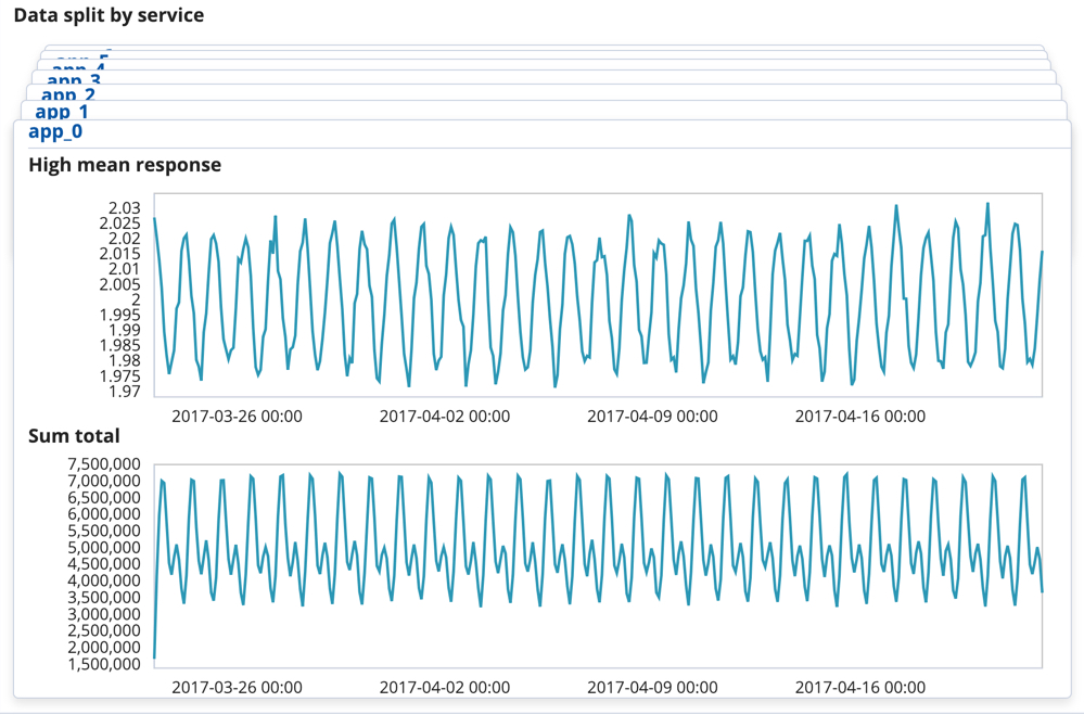
-
Provide a name for the job, for example
response_requests_by_app. The job name must be unique in your cluster. You can also optionally provide a description of the job. - Click Create Job.
When the job is created, you can choose to view the results, continue the job in real-time, and create a watch. In this tutorial, we will proceed to view the results.
The create_multi_metric.sh script, which is included with the
sample data, creates a similar job and datafeed by
using the machine learning APIs. Before you run it, you must edit the USERNAME and PASSWORD
variables with your actual user ID and password. If the Elasticsearch security features
are not enabled, use the create_multi_metric_noauth.sh script instead. For API
reference information, see Machine Learning APIs.