Term join
editTerm join
editUse term joins to augment vector features with properties for data driven styling and richer tooltip content.
Term joins are available for vector layers with the following sources:
- Custom vector shapes
- Documents
- Vector shapes
Example term join
editThe choropleth layer example uses a term join to shade world countries by web log traffic. Darker shades symbolize countries with more web log traffic, and lighter shades symbolize countries with less traffic.
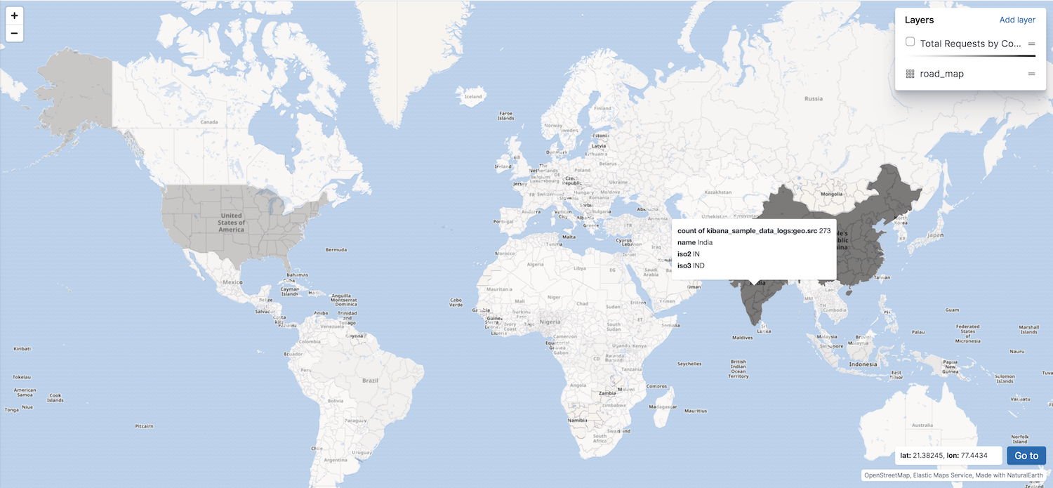
How a term join works
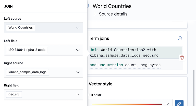
editA term join uses a shared key to combine vector features, the left source, with the results of an Elasticsearch terms aggregation, the right source.
The cloropeth example uses the shared key, ISO 3166-1 alpha-2 code, to join world countries and web log traffic. ISO 3166-1 alpha-2 code is an international standard that identifies countries by a two-letter country code. For example, Sweden has an ISO 3166-1 alpha-2 code of SE.
Left source
editThe left source for the term join is the Elastic Maps Service (EMS) World Countries. Vector features for this source are provided by EMS. You can also use your own vector features.
In the following example, iso2 property defines the shared key for the left source.
{
  geometry: {
    coordinates: [...],
    type: "Polygon"
  },
  properties: {
    name: "Sweden",
    iso2: "SE"
  },
  type: "Feature"
}
Right source
editThe right source uses the Kibana sample data set "Sample web logs". In this data set, the geo.src field contains the ISO 3166-1 alpha-2 code of the country of origin.
A terms aggregation groups the sample web log documents by geo.src and calculates metrics for each term.
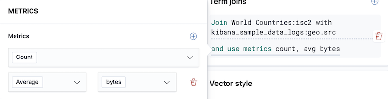
The METRICS configuration defines two metric aggregations:
- The count of all documents in the terms bucket.
- The average of the field "bytes" for all documents in the terms bucket.
The right source does not provide individual documents, but instead provides the metrics from a terms aggregation. The metrics are calculated from the following sample web logs documents.
{
  bytes: 1837,
  geo: {
    src: "SE"
  },
  timestamp: "Feb 28, 2019 @ 07:23:08.754"
},
{
  bytes: 971,
  geo: {
    src: "SE"
  },
  timestamp: "Feb 27, 2019 @ 08:10:45.205"
},
{
  bytes: 4277,
  geo: {
    src: "SE"
  },
  timestamp: "Feb 21, 2019 @ 05:24:33.945"
},
{
  bytes: 5624,
  geo: {
    src: "SE"
  },
  timestamp: "Feb 21, 2019 @ 04:57:05.921"
}
The terms aggregation creates a bucket for each unique geo.src value. Metrics are calucated for all documents in a bucket.
The following shows an example terms aggregation response. Note the key property, which defines the shared key for the right source.
{
  aggregations: {
    join: {
      buckets: [
        {
          doc_count: 4,
          key: "SE",
          avg_of_bytes: {
            value: 3177.25
          }
        },
        ...
      ]
    }
  }
}
Augmenting the left source with metrics from the right source
editThe join adds metrics for each terms aggregation bucket to the world country feature with the corresponding ISO 3166-1 alpha-2 code. Features that do not have a corresponding terms aggregation bucket are not visible on the map.
The world country features now have two additional properties:
- Count of web log traffic originating from the world country
- Average bytes of web log traffic originating from the world country
The cloropeth example uses the count of web log traffic to symbolize countries by web log traffic.