WARNING: Version 6.0 of Elasticsearch has passed its EOL date.
This documentation is no longer being maintained and may be removed. If you are running this version, we strongly advise you to upgrade. For the latest information, see the current release documentation.
Moving Average Aggregation
editMoving Average Aggregation
editGiven an ordered series of data, the Moving Average aggregation will slide a window across the data and emit the average
value of that window. For example, given the data [1, 2, 3, 4, 5, 6, 7, 8, 9, 10], we can calculate a simple moving
average with windows size of 5 as follows:
- (1 + 2 + 3 + 4 + 5) / 5 = 3
- (2 + 3 + 4 + 5 + 6) / 5 = 4
- (3 + 4 + 5 + 6 + 7) / 5 = 5
- etc
Moving averages are a simple method to smooth sequential data. Moving averages are typically applied to time-based data, such as stock prices or server metrics. The smoothing can be used to eliminate high frequency fluctuations or random noise, which allows the lower frequency trends to be more easily visualized, such as seasonality.
Syntax
editA moving_avg aggregation looks like this in isolation:
{
    "moving_avg": {
        "buckets_path": "the_sum",
        "model": "holt",
        "window": 5,
        "gap_policy": "insert_zeros",
        "settings": {
            "alpha": 0.8
        }
    }
}
Table 9. moving_avg Parameters
Parameter Name |
Description |
Required |
Default Value |
|
Path to the metric of interest (see |
Required |
|
|
The moving average weighting model that we wish to use |
Optional |
|
|
Determines what should happen when a gap in the data is encountered. |
Optional |
|
|
The size of window to "slide" across the histogram. |
Optional |
|
|
If the model should be algorithmically minimized. See Minimization for more details |
Optional |
|
|
Model-specific settings, contents which differ depending on the model specified. |
Optional |
moving_avg aggregations must be embedded inside of a histogram or date_histogram aggregation. They can be
embedded like any other metric aggregation:
POST /_search
{
    "size": 0,
    "aggs": {
        "my_date_histo":{
            "date_histogram":{
                "field":"date",
                "interval":"1M"
            },
            "aggs":{
                "the_sum":{
                    "sum":{ "field": "price" }
                },
                "the_movavg":{
                    "moving_avg":{ "buckets_path": "the_sum" }
                }
            }
        }
    }
}
|
A |
|
|
A |
|
|
Finally, we specify a |
Moving averages are built by first specifying a histogram or date_histogram over a field. You can then optionally
add normal metrics, such as a sum, inside of that histogram. Finally, the moving_avg is embedded inside the histogram.
The buckets_path parameter is then used to "point" at one of the sibling metrics inside of the histogram (see
buckets_path Syntax for a description of the syntax for buckets_path.
An example response from the above aggregation may look like:
{
   "took": 11,
   "timed_out": false,
   "_shards": ...,
   "hits": ...,
   "aggregations": {
      "my_date_histo": {
         "buckets": [
             {
                 "key_as_string": "2015/01/01 00:00:00",
                 "key": 1420070400000,
                 "doc_count": 3,
                 "the_sum": {
                    "value": 550.0
                 }
             },
             {
                 "key_as_string": "2015/02/01 00:00:00",
                 "key": 1422748800000,
                 "doc_count": 2,
                 "the_sum": {
                    "value": 60.0
                 },
                 "the_movavg": {
                    "value": 550.0
                 }
             },
             {
                 "key_as_string": "2015/03/01 00:00:00",
                 "key": 1425168000000,
                 "doc_count": 2,
                 "the_sum": {
                    "value": 375.0
                 },
                 "the_movavg": {
                    "value": 305.0
                 }
             }
         ]
      }
   }
}
Models
editThe moving_avg aggregation includes four different moving average "models". The main difference is how the values in the
window are weighted. As data-points become "older" in the window, they may be weighted differently. This will
affect the final average for that window.
Models are specified using the model parameter. Some models may have optional configurations which are specified inside
the settings parameter.
Simple
editThe simple model calculates the sum of all values in the window, then divides by the size of the window. It is effectively
a simple arithmetic mean of the window. The simple model does not perform any time-dependent weighting, which means
the values from a simple moving average tend to "lag" behind the real data.
POST /_search
{
    "size": 0,
    "aggs": {
        "my_date_histo":{
            "date_histogram":{
                "field":"date",
                "interval":"1M"
            },
            "aggs":{
                "the_sum":{
                    "sum":{ "field": "price" }
                },
                "the_movavg":{
                    "moving_avg":{
                        "buckets_path": "the_sum",
                        "window" : 30,
                        "model" : "simple"
                    }
                }
            }
        }
    }
}
A simple model has no special settings to configure
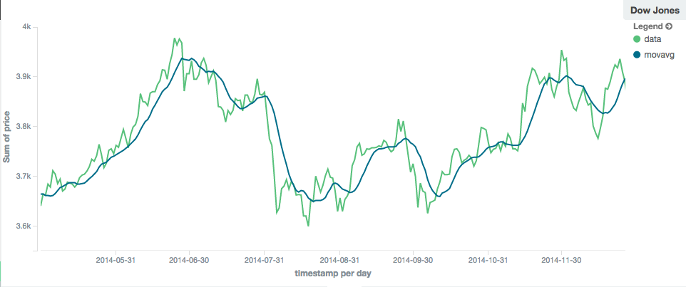
The window size can change the behavior of the moving average. For example, a small window ("window": 10) will closely
track the data and only smooth out small scale fluctuations:
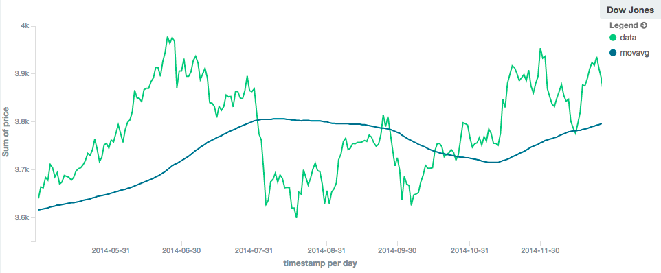
In contrast, a simple moving average with larger window ("window": 100) will smooth out all higher-frequency fluctuations,
leaving only low-frequency, long term trends. It also tends to "lag" behind the actual data by a substantial amount:
Linear
editThe linear model assigns a linear weighting to points in the series, such that "older" datapoints (e.g. those at
the beginning of the window) contribute a linearly less amount to the total average. The linear weighting helps reduce
the "lag" behind the data’s mean, since older points have less influence.
POST /_search
{
    "size": 0,
    "aggs": {
        "my_date_histo":{
            "date_histogram":{
                "field":"date",
                "interval":"1M"
            },
            "aggs":{
                "the_sum":{
                    "sum":{ "field": "price" }
                },
                "the_movavg": {
                    "moving_avg":{
                        "buckets_path": "the_sum",
                        "window" : 30,
                        "model" : "linear"
                    }
                }
            }
        }
    }
}
A linear model has no special settings to configure
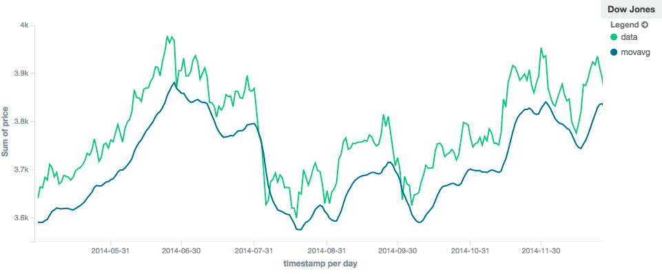
Like the simple model, window size can change the behavior of the moving average. For example, a small window ("window": 10)
will closely track the data and only smooth out small scale fluctuations:
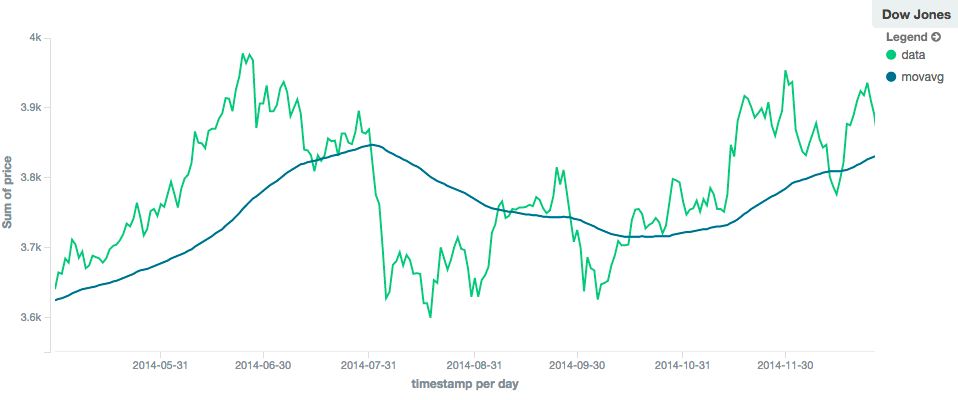
In contrast, a linear moving average with larger window ("window": 100) will smooth out all higher-frequency fluctuations,
leaving only low-frequency, long term trends. It also tends to "lag" behind the actual data by a substantial amount,
although typically less than the simple model:
EWMA (Exponentially Weighted)
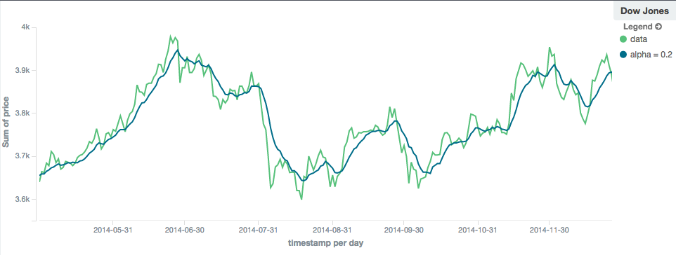
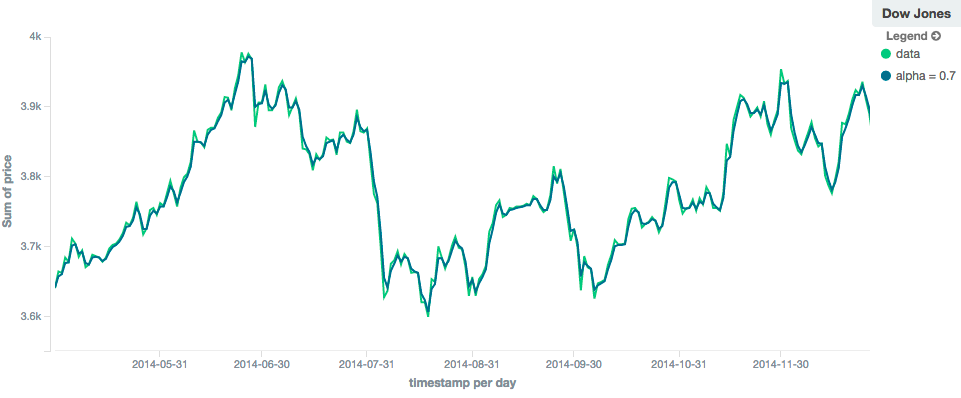
editThe ewma model (aka "single-exponential") is similar to the linear model, except older data-points become exponentially less important,
rather than linearly less important. The speed at which the importance decays can be controlled with an alpha
setting. Small values make the weight decay slowly, which provides greater smoothing and takes into account a larger
portion of the window. Larger valuers make the weight decay quickly, which reduces the impact of older values on the
moving average. This tends to make the moving average track the data more closely but with less smoothing.
The default value of alpha is 0.3, and the setting accepts any float from 0-1 inclusive.
The EWMA model can be Minimized
POST /_search
{
    "size": 0,
    "aggs": {
        "my_date_histo":{
            "date_histogram":{
                "field":"date",
                "interval":"1M"
            },
            "aggs":{
                "the_sum":{
                    "sum":{ "field": "price" }
                },
                "the_movavg": {
                    "moving_avg":{
                        "buckets_path": "the_sum",
                        "window" : 30,
                        "model" : "ewma",
                        "settings" : {
                            "alpha" : 0.5
                        }
                    }
                }
            }
        }
    }
}
Holt-Linear
editThe holt model (aka "double exponential") incorporates a second exponential term which
tracks the data’s trend. Single exponential does not perform well when the data has an underlying linear trend. The
double exponential model calculates two values internally: a "level" and a "trend".
The level calculation is similar to ewma, and is an exponentially weighted view of the data. The difference is
that the previously smoothed value is used instead of the raw value, which allows it to stay close to the original series.
The trend calculation looks at the difference between the current and last value (e.g. the slope, or trend, of the
smoothed data). The trend value is also exponentially weighted.
Values are produced by multiplying the level and trend components.
The default value of alpha is 0.3 and beta is 0.1. The settings accept any float from 0-1 inclusive.
The Holt-Linear model can be Minimized
POST /_search
{
    "size": 0,
    "aggs": {
        "my_date_histo":{
            "date_histogram":{
                "field":"date",
                "interval":"1M"
            },
            "aggs":{
                "the_sum":{
                    "sum":{ "field": "price" }
                },
                "the_movavg": {
                    "moving_avg":{
                        "buckets_path": "the_sum",
                        "window" : 30,
                        "model" : "holt",
                        "settings" : {
                            "alpha" : 0.5,
                            "beta" : 0.5
                        }
                    }
                }
            }
        }
    }
}
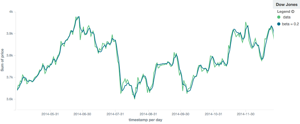
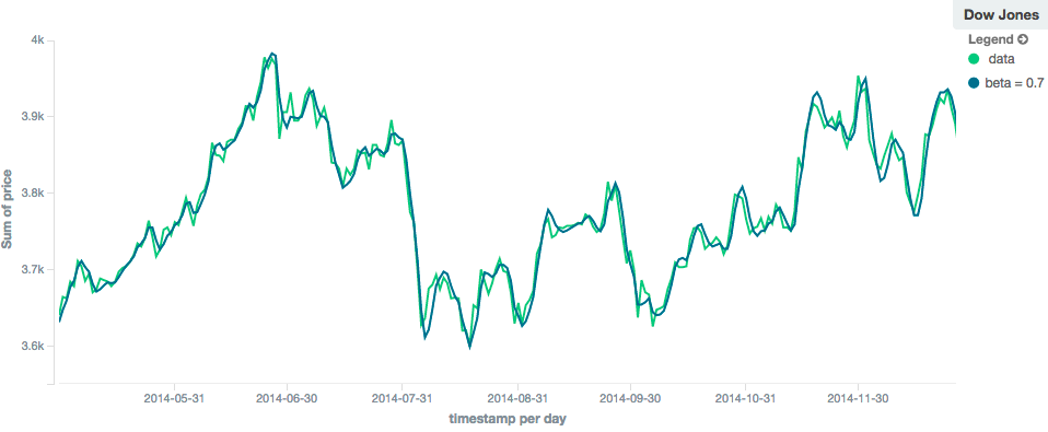
In practice, the alpha value behaves very similarly in holt as ewma: small values produce more smoothing
and more lag, while larger values produce closer tracking and less lag. The value of beta is often difficult
to see. Small values emphasize long-term trends (such as a constant linear trend in the whole series), while larger
values emphasize short-term trends. This will become more apparently when you are predicting values.
Holt-Winters
editThe holt_winters model (aka "triple exponential") incorporates a third exponential term which
tracks the seasonal aspect of your data. This aggregation therefore smooths based on three components: "level", "trend"
and "seasonality".
The level and trend calculation is identical to holt The seasonal calculation looks at the difference between
the current point, and the point one period earlier.
Holt-Winters requires a little more handholding than the other moving averages. You need to specify the "periodicity"
of your data: e.g. if your data has cyclic trends every 7 days, you would set period: 7. Similarly if there was
a monthly trend, you would set it to 30. There is currently no periodicity detection, although that is planned
for future enhancements.
There are two varieties of Holt-Winters: additive and multiplicative.
"Cold Start"
editUnfortunately, due to the nature of Holt-Winters, it requires two periods of data to "bootstrap" the algorithm. This
means that your window must always be at least twice the size of your period. An exception will be thrown if it
isn’t. It also means that Holt-Winters will not emit a value for the first 2 * period buckets; the current algorithm
does not backcast.
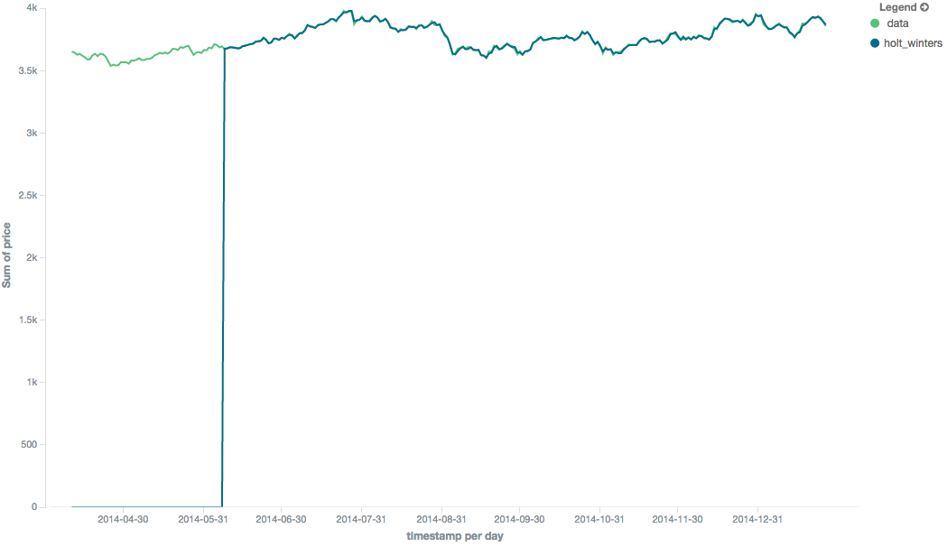
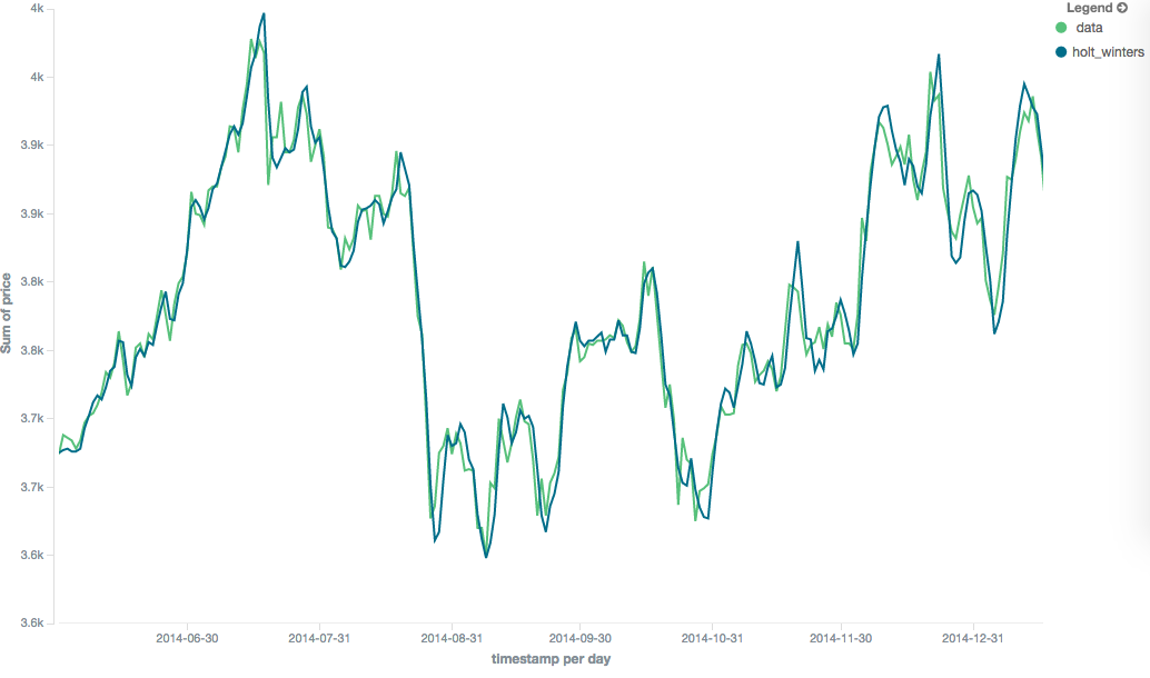
Because the "cold start" obscures what the moving average looks like, the rest of the Holt-Winters images are truncated to not show the "cold start". Just be aware this will always be present at the beginning of your moving averages!
Additive Holt-Winters
editAdditive seasonality is the default; it can also be specified by setting "type": "add". This variety is preferred
when the seasonal affect is additive to your data. E.g. you could simply subtract the seasonal effect to "de-seasonalize"
your data into a flat trend.
The default values of alpha and gamma are 0.3 while beta is 0.1. The settings accept any float from 0-1 inclusive.
The default value of period is 1.
The additive Holt-Winters model can be Minimized
POST /_search
{
    "size": 0,
    "aggs": {
        "my_date_histo":{
            "date_histogram":{
                "field":"date",
                "interval":"1M"
            },
            "aggs":{
                "the_sum":{
                    "sum":{ "field": "price" }
                },
                "the_movavg": {
                    "moving_avg":{
                        "buckets_path": "the_sum",
                        "window" : 30,
                        "model" : "holt_winters",
                        "settings" : {
                            "type" : "add",
                            "alpha" : 0.5,
                            "beta" : 0.5,
                            "gamma" : 0.5,
                            "period" : 7
                        }
                    }
                }
            }
        }
    }
}
Multiplicative Holt-Winters
editMultiplicative is specified by setting "type": "mult". This variety is preferred when the seasonal affect is
multiplied against your data. E.g. if the seasonal affect is x5 the data, rather than simply adding to it.
The default values of alpha and gamma are 0.3 while beta is 0.1. The settings accept any float from 0-1 inclusive.
The default value of period is 1.
The multiplicative Holt-Winters model can be Minimized
Multiplicative Holt-Winters works by dividing each data point by the seasonal value. This is problematic if any of
your data is zero, or if there are gaps in the data (since this results in a divid-by-zero). To combat this, the
mult Holt-Winters pads all values by a very small amount (1*10-10) so that all values are non-zero. This affects
the result, but only minimally. If your data is non-zero, or you prefer to see NaN when zero’s are encountered,
you can disable this behavior with pad: false
POST /_search
{
    "size": 0,
    "aggs": {
        "my_date_histo":{
            "date_histogram":{
                "field":"date",
                "interval":"1M"
            },
            "aggs":{
                "the_sum":{
                    "sum":{ "field": "price" }
                },
                "the_movavg": {
                    "moving_avg":{
                        "buckets_path": "the_sum",
                        "window" : 30,
                        "model" : "holt_winters",
                        "settings" : {
                            "type" : "mult",
                            "alpha" : 0.5,
                            "beta" : 0.5,
                            "gamma" : 0.5,
                            "period" : 7,
                            "pad" : true
                        }
                    }
                }
            }
        }
    }
}
Prediction
editThis functionality is in technical preview and may be changed or removed in a future release. Elastic will work to fix any issues, but features in technical preview are not subject to the support SLA of official GA features.
All the moving average model support a "prediction" mode, which will attempt to extrapolate into the future given the current smoothed, moving average. Depending on the model and parameter, these predictions may or may not be accurate.
Predictions are enabled by adding a predict parameter to any moving average aggregation, specifying the number of
predictions you would like appended to the end of the series. These predictions will be spaced out at the same interval
as your buckets:
POST /_search
{
    "size": 0,
    "aggs": {
        "my_date_histo":{
            "date_histogram":{
                "field":"date",
                "interval":"1M"
            },
            "aggs":{
                "the_sum":{
                    "sum":{ "field": "price" }
                },
                "the_movavg": {
                    "moving_avg":{
                        "buckets_path": "the_sum",
                        "window" : 30,
                        "model" : "simple",
                        "predict" : 10
                    }
                }
            }
        }
    }
}
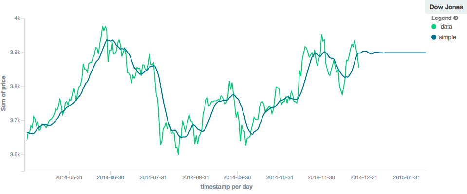
The simple, linear and ewma models all produce "flat" predictions: they essentially converge on the mean
of the last value in the series, producing a flat:
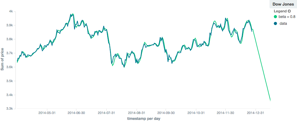
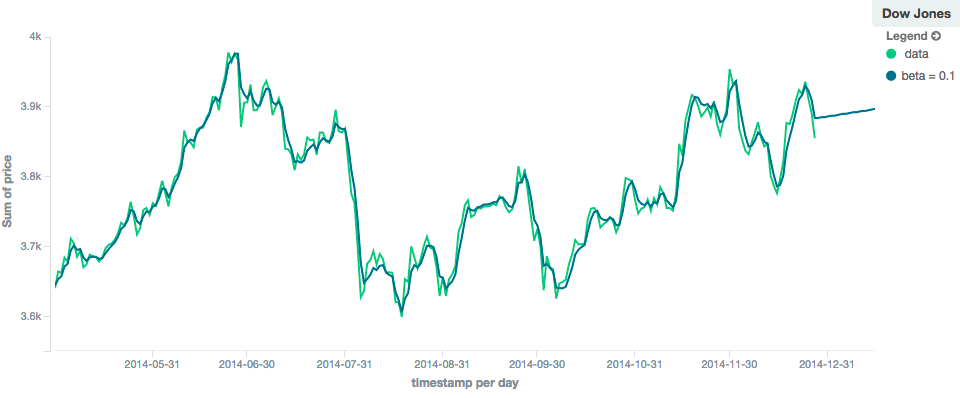
In contrast, the holt model can extrapolate based on local or global constant trends. If we set a high beta
value, we can extrapolate based on local constant trends (in this case the predictions head down, because the data at the end
of the series was heading in a downward direction):
In contrast, if we choose a small beta, the predictions are based on the global constant trend. In this series, the
global trend is slightly positive, so the prediction makes a sharp u-turn and begins a positive slope:
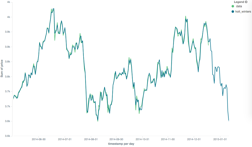
The holt_winters model has the potential to deliver the best predictions, since it also incorporates seasonal
fluctuations into the model:
Minimization
editSome of the models (EWMA, Holt-Linear, Holt-Winters) require one or more parameters to be configured. Parameter choice can be tricky and sometimes non-intuitive. Furthermore, small deviations in these parameters can sometimes have a drastic effect on the output moving average.
For that reason, the three "tunable" models can be algorithmically minimized. Minimization is a process where parameters are tweaked until the predictions generated by the model closely match the output data. Minimization is not fullproof and can be susceptible to overfitting, but it often gives better results than hand-tuning.
Minimization is disabled by default for ewma and holt_linear, while it is enabled by default for holt_winters.
Minimization is most useful with Holt-Winters, since it helps improve the accuracy of the predictions. EWMA and
Holt-Linear are not great predictors, and mostly used for smoothing data, so minimization is less useful on those
models.
Minimization is enabled/disabled via the minimize parameter:
POST /_search
{
    "size": 0,
    "aggs": {
        "my_date_histo":{
            "date_histogram":{
                "field":"date",
                "interval":"1M"
            },
            "aggs":{
                "the_sum":{
                    "sum":{ "field": "price" }
                },
                "the_movavg": {
                    "moving_avg":{
                        "buckets_path": "the_sum",
                        "model" : "holt_winters",
                        "window" : 30,
                        "minimize" : true,
                        "settings" : {
                            "period" : 7
                        }
                    }
                }
            }
        }
    }
}
When enabled, minimization will find the optimal values for alpha, beta and gamma. The user should still provide
appropriate values for window, period and type.
Minimization works by running a stochastic process called simulated annealing. This process will usually generate a good solution, but is not guaranteed to find the global optimum. It also requires some amount of additional computational power, since the model needs to be re-run multiple times as the values are tweaked. The run-time of minimization is linear to the size of the window being processed: excessively large windows may cause latency.
Finally, minimization fits the model to the last n values, where n = window. This generally produces
better forecasts into the future, since the parameters are tuned around the end of the series. It can, however, generate
poorer fitting moving averages at the beginning of the series.