WARNING: The 2.x versions of Elasticsearch have passed their EOL dates. If you are running a 2.x version, we strongly advise you to upgrade.
This documentation is no longer maintained and may be removed. For the latest information, see the current Elasticsearch documentation.
Calculating Percentiles
editCalculating Percentilesedit
The other approximate metric offered by Elasticsearch is the percentiles metric.
Percentiles show the point at which a certain percentage of observed values occur.
For example, the 95th percentile is the value that is greater than 95% of the
data.
Percentiles are often used to find outliers. In (statistically) normal distributions, the 0.13th and 99.87th percentiles represent three standard deviations from the mean. Any data that falls outside three standard deviations is often considered an anomaly because it is so different from the average value.
To be more concrete, imagine that you are running a large website and it is your job to guarantee fast response times to visitors. You must therefore monitor your website latency to determine whether you are meeting your goal.
A common metric to use in this scenario is the average latency. But this is a poor choice (despite being common), because averages can easily hide outliers. A median metric also suffers the same problem. You could try a maximum, but this metric is easily skewed by just a single outlier.
This graph in Figure 40, “Average request latency over time” visualizes the problem. If you rely on simple metrics like mean or median, you might see a graph that looks like Figure 40, “Average request latency over time”.
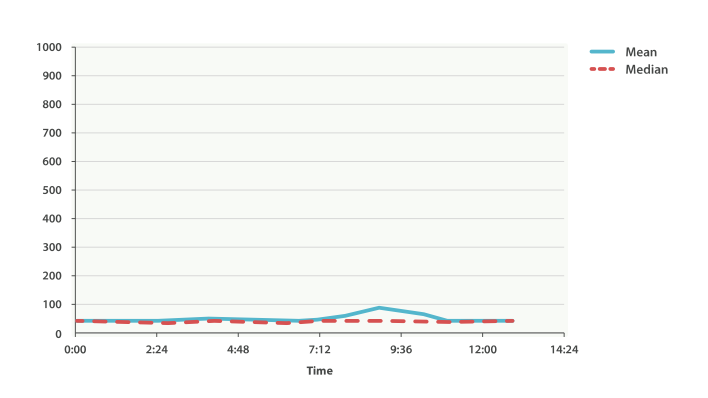
Everything looks fine. There is a slight bump, but nothing to be concerned about. But if we load up the 99th percentile (the value that accounts for the slowest 1% of latencies), we see an entirely different story, as shown in Figure 41, “Average request latency with 99th percentile over time”.
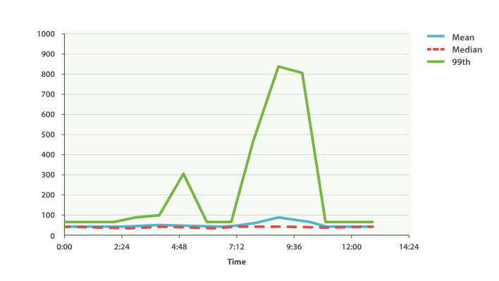
Whoa! At 9:30 a.m., the mean is only 75ms. As a system administrator, you wouldn’t look at this value twice. Everything normal! But the 99th percentile is telling you that 1% of your customers are seeing latency in excess of 850ms—a very different story. There is also a smaller spike at 4:48 a.m. that wasn’t even noticeable in the mean/median.
This is just one use-case for a percentile. Percentiles can also be used to quickly eyeball the distribution of data, check for skew or bimodalities, and more.
Percentile Metricedit
Let’s load a new dataset (the car data isn’t going to work well for percentiles). We are going to index a bunch of website latencies and run a few percentiles over it:
POST /website/logs/_bulk
{ "index": {}}
{ "latency" : 100, "zone" : "US", "timestamp" : "2014-10-28" }
{ "index": {}}
{ "latency" : 80, "zone" : "US", "timestamp" : "2014-10-29" }
{ "index": {}}
{ "latency" : 99, "zone" : "US", "timestamp" : "2014-10-29" }
{ "index": {}}
{ "latency" : 102, "zone" : "US", "timestamp" : "2014-10-28" }
{ "index": {}}
{ "latency" : 75, "zone" : "US", "timestamp" : "2014-10-28" }
{ "index": {}}
{ "latency" : 82, "zone" : "US", "timestamp" : "2014-10-29" }
{ "index": {}}
{ "latency" : 100, "zone" : "EU", "timestamp" : "2014-10-28" }
{ "index": {}}
{ "latency" : 280, "zone" : "EU", "timestamp" : "2014-10-29" }
{ "index": {}}
{ "latency" : 155, "zone" : "EU", "timestamp" : "2014-10-29" }
{ "index": {}}
{ "latency" : 623, "zone" : "EU", "timestamp" : "2014-10-28" }
{ "index": {}}
{ "latency" : 380, "zone" : "EU", "timestamp" : "2014-10-28" }
{ "index": {}}
{ "latency" : 319, "zone" : "EU", "timestamp" : "2014-10-29" }
This data contains three values: a latency, a data center zone, and a date
timestamp. Let’s run percentiles over the whole dataset to get a feel for
the distribution:
GET /website/logs/_search
{
    "size" : 0,
    "aggs" : {
        "load_times" : {
            "percentiles" : {
                "field" : "latency"
            }
        },
        "avg_load_time" : {
            "avg" : {
                "field" : "latency"
            }
        }
    }
}
|
The |
|
|
For comparison, we also execute an |
By default, the percentiles metric will return an array of predefined percentiles:
[1, 5, 25, 50, 75, 95, 99]. These represent common percentiles that people are
interested in—the extreme percentiles at either end of the spectrum, and a
few in the middle. In the response, we see that the fastest latency is around 75ms,
while the slowest is almost 600ms. In contrast, the average is sitting near
200ms, which is much less informative:
...
"aggregations": {
  "load_times": {
     "values": {
        "1.0": 75.55,
        "5.0": 77.75,
        "25.0": 94.75,
        "50.0": 101,
        "75.0": 289.75,
        "95.0": 489.34999999999985,
        "99.0": 596.2700000000002
     }
  },
  "avg_load_time": {
     "value": 199.58333333333334
  }
}
So there is clearly a wide distribution in latencies. Let’s see whether it is correlated to the geographic zone of the data center:
GET /website/logs/_search
{
    "size" : 0,
    "aggs" : {
        "zones" : {
            "terms" : {
                "field" : "zone"
            },
            "aggs" : {
                "load_times" : {
                    "percentiles" : {
                      "field" : "latency",
                      "percents" : [50, 95.0, 99.0]
                    }
                },
                "load_avg" : {
                    "avg" : {
                        "field" : "latency"
                    }
                }
            }
        }
    }
}
|
First we separate our latencies into buckets, depending on their zone. |
|
|
Then we calculate the percentiles per zone. |
|
|
The |
From the response, we can see the EU zone is much slower than the US zone. On the US side, the 50th percentile is very close to the 99th percentile—and both are close to the average.
In contrast, the EU zone has a large difference between the 50th and 99th percentile. It is now obvious that the EU zone is dragging down the latency statistics, and we know that 50% of the EU zone is seeing 300ms+ latencies.
...
"aggregations": {
  "zones": {
     "buckets": [
        {
           "key": "eu",
           "doc_count": 6,
           "load_times": {
              "values": {
                 "50.0": 299.5,
                 "95.0": 562.25,
                 "99.0": 610.85
              }
           },
           "load_avg": {
              "value": 309.5
           }
        },
        {
           "key": "us",
           "doc_count": 6,
           "load_times": {
              "values": {
                 "50.0": 90.5,
                 "95.0": 101.5,
                 "99.0": 101.9
              }
           },
           "load_avg": {
              "value": 89.66666666666667
           }
        }
     ]
  }
}
...
Percentile Ranksedit
There is another, closely related metric called percentile_ranks. The
percentiles metric tells you the lowest value below which a given percentage of documents fall. For instance, if the 50th percentile is 119ms, then 50% of documents have values of no more than 119ms. The percentile_ranks tells you which percentile a specific value belongs to. The percentile_ranks of 119ms is the 50th percentile. It is basically a two-way relationship. For example:
- The 50th percentile is 119ms.
- The 119ms percentile rank is the 50th percentile.
So imagine that our website must maintain an SLA of 210ms response times or less. And, just for fun, your boss has threatened to fire you if response times creep over 800ms. Understandably, you would like to know what percentage of requests are actually meeting that SLA (and hopefully at least under 800ms!).
For this, you can apply the percentile_ranks metric instead of percentiles:
GET /website/logs/_search
{
    "size" : 0,
    "aggs" : {
        "zones" : {
            "terms" : {
                "field" : "zone"
            },
            "aggs" : {
                "load_times" : {
                    "percentile_ranks" : {
                      "field" : "latency",
                      "values" : [210, 800]
                    }
                }
            }
        }
    }
}
After running this aggregation, we get two values back:
"aggregations": {
  "zones": {
     "buckets": [
        {
           "key": "eu",
           "doc_count": 6,
           "load_times": {
              "values": {
                 "210.0": 31.944444444444443,
                 "800.0": 100
              }
           }
        },
        {
           "key": "us",
           "doc_count": 6,
           "load_times": {
              "values": {
                 "210.0": 100,
                 "800.0": 100
              }
           }
        }
     ]
  }
}
This tells us three important things:
- In the EU zone, the percentile rank for 210ms is 31.94%.
- In the US zone, the percentile rank for 210ms is 100%.
- In both EU and US, the percentile rank for 800ms is 100%.
In plain english, this means that the EU zone is meeting the SLA only 32% of the time, while the US zone is always meeting the SLA. But luckily for you, both zones are under 800ms, so you won’t be fired (yet!).
The percentile_ranks metric provides the same information as percentiles, but
presented in a different format that may be more convenient if you are interested in specific value(s).
Understanding the Trade-offsedit
Like cardinality, calculating percentiles requires an approximate algorithm. The naive implementation would maintain a sorted list of all values—but this clearly is not possible when you have billions of values distributed across dozens of nodes.
Instead, percentiles uses an algorithm called TDigest (introduced by Ted Dunning
in Computing Extremely Accurate Quantiles Using T-Digests). As with HyperLogLog, it isn’t
necessary to understand the full technical details, but it is good to know
the properties of the algorithm:
- Percentile accuracy is proportional to how extreme the percentile is. This means that percentiles such as the 1st or 99th are more accurate than the 50th. This is just a property of how the data structure works, but it happens to be a nice property, because most people care about extreme percentiles.
- For small sets of values, percentiles are highly accurate. If the dataset is small enough, the percentiles may be 100% exact.
- As the quantity of values in a bucket grows, the algorithm begins to approximate the percentiles. It is effectively trading accuracy for memory savings. The exact level of inaccuracy is difficult to generalize, since it depends on your data distribution and volume of data being aggregated.
Similar to cardinality, you can control the memory-to-accuracy ratio by changing
a parameter: compression.
The TDigest algorithm uses nodes to approximate percentiles: the more nodes available, the higher the accuracy (and the larger the memory footprint)
proportional to the volume of data. The compression parameter limits the maximum
number of nodes to 20 * compression.
Therefore, by increasing the compression value, you can increase the accuracy of
your percentiles at the cost of more memory. Larger compression values also
make the algorithm slower since the underlying tree data structure grows in size, resulting in more expensive operations. The default compression value is 100.
A node uses roughly 32 bytes of memory, so in a worst-case scenario (for example, a large amount of data that arrives sorted and in order), the default settings will produce a TDigest roughly 64KB in size. In practice, data tends to be more random, and the TDigest will use less memory.