REST API
editREST API
editGraph Explore API
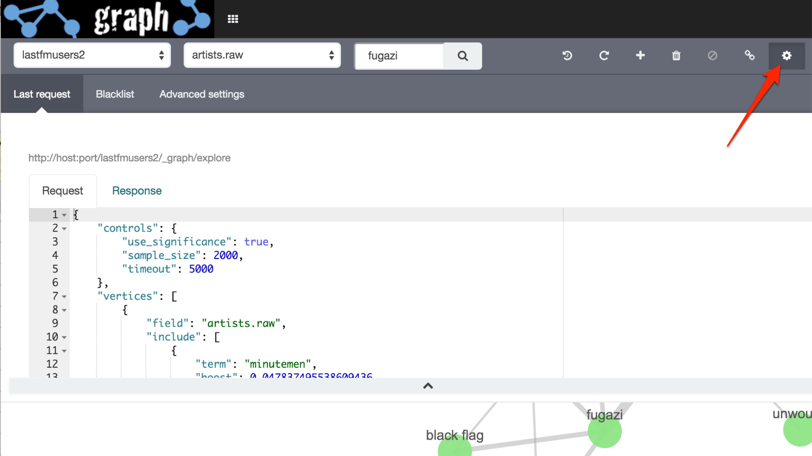
editThe Graph "explore" API is accessible via the /_graph/explore endpoint. One of the best ways to understand the behaviour of this API is to use the Kibana graph plugin to visually click around connected data and then view the "Last request" panel (accessible from the button with the cog icon). This panel shows the JSON request/response pair of the last user operation.
Basic exploration
editAn initial search typically begins with a query to identify strongly related terms.
POST clicklogs/_graph/explore
{
    "query": {
        "match": {
            "query.raw": "midi"
        }
    },
    "vertices": [
        {
            "field": "product"
        }
    ],
    "connections": {
        "vertices": [
            {
                "field": "query.raw"
            }
        ]
    }
}
|
A query is used to "seed" the exploration - here we are looking in clicklogs for people who searched for "midi". Any of the usual elasticsearch query syntax can be used here to identify the documents of interest. |
|
|
A list of fields is provided - here we want to find product codes that are significantly associated with searches for "midi" |
|
|
A list of fields is provided again - here we are looking for other search terms that led people to click on the products found in 2) |
Further "connections" can be nested inside the "connections" object to continue exploring out the relationships in the data. Each level of nesting is commonly referred to as a "hop" and proximity in a graph is often thought of in terms of "hop depth".
The response from a graph exploration is as follows:
{
   "took": 0,
   "timed_out": false,
   "failures": [],
   "vertices": [
      {
         "field": "query.raw",
         "term": "midi cable",
         "weight": 0.08745858139552132,
         "depth": 1
      },
      {
         "field": "product",
         "term": "8567446",
         "weight": 0.13247784285434397,
         "depth": 0
      },
      {
         "field": "product",
         "term": "1112375",
         "weight": 0.018600718471158982,
         "depth": 0
      },
      {
         "field": "query.raw",
         "term": "midi keyboard",
         "weight": 0.04802242866755111,
         "depth": 1
      }
   ],
   "connections": [
      {
         "source": 0,
         "target": 1,
         "weight": 0.04802242866755111,
         "doc_count": 13
      },
      {
         "source": 2,
         "target": 3,
         "weight": 0.08120623870976627,
         "doc_count": 23
      }
   ]
}
|
An array of all of the vertices that were discovered. A vertex is an indexed term so the field and term value are supplied. The |
|
|
The connections between the vertices in the array. The |
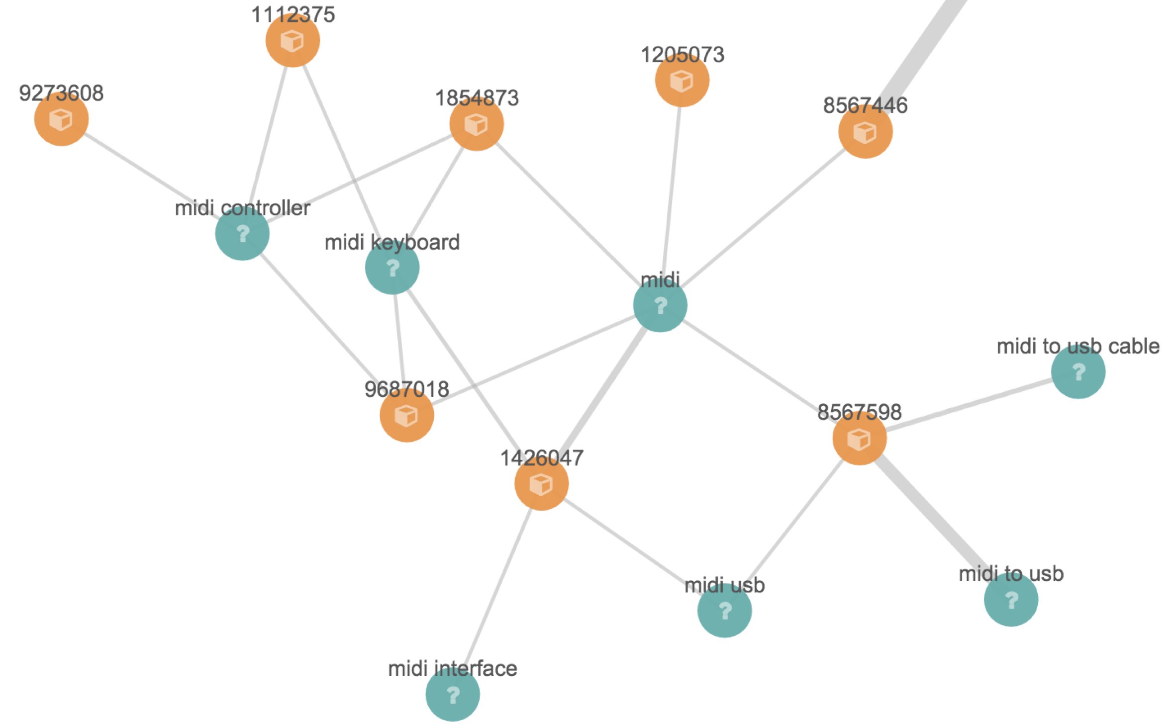
In the Kibana Graph plugin app response data is visualized in a diagram like this:
Optional controls
editThe previous basic example omitted several parameters that have default values. This fuller example illustrates the additional parameters that can be used in graph explore requests.
POST clicklogs/_graph/explore
{
   "query": {
      "bool": {
         "must": {
            "match": {
               "query.raw": "midi"
            }
         },
         "filter": [
            {
               "range": {
                  "query_time": {
                     "gte": "2015-10-01 00:00:00"
                  }
               }
            }
         ]
      }
   },
   "controls": {
      "use_significance": true,
      "sample_size": 2000,
      "timeout": 2000,
      "sample_diversity": {
         "field": "category.raw",
         "max_docs_per_value": 500
      }
   },
   "vertices": [
      {
         "field": "product",
         "size": 5,
         "min_doc_count": 10,
         "shard_min_doc_count": 3
      }
   ],
   "connections": {
      "query": {
         "bool": {
            "filter": [
               {
                  "range": {
                     "query_time": {
                        "gte": "2015-10-01 00:00:00"
                     }
                  }
               }
            ]
         }
      },
      "vertices": [
         {
            "field": "query.raw",
            "size": 5,
            "min_doc_count": 10,
            "shard_min_doc_count": 3
         }
      ]
   }
}
|
This seed query iin this example is a more complex query for the word "midi" but with a date filter. |
|
|
The |
|
|
Each "hop" considers a sample of the best-matching documents on each shard (default is 100 documents). Using samples has the dual benefit of keeping exploration focused on meaningfully-connected terms and improving the speed of execution. Very small values (less than 50) may not provide sufficient weight-of-evidence to identify significant connections between terms while very large sample sizes may dilute the quality and be slow. |
|
|
A |
|
|
To avoid the top-matching documents sample being dominated by a single source of results sometimes it can prove necessary to request diversity in the sample. This is achieved by selecting a single-value field and a maximum number of documents per value in that field. In this example we are requiring that there are no more than 500 click documents from any one department in the store. This might help us consider products from the electronics, book and video departments whereas without this diversification our results may be entirely dominated by the electronics department. |
|
|
We can control the maximum number of vertex terms returned for each field using the |
|
|
|
|
|
|
|
|
Optionally, a "guiding query" can be used to guide the Graph API as it explores connected terms. In this case we are guiding the hop from products to related queries by only considering documents that are also clicks that have been recorded recently. |
The default settings are configured to remove noisy data and get "the big picture" from data. For more detailed forensic type work where every document could be of interest see the troubleshooting guide for tips on tuning the settings for this type of work.
"Spidering" operations
editAfter an initial search users typically want to review the results using a form of graph visualization tool like the one in the Kibana graph plugin. Users will frequently then select one or more vertices of interest and ask to load more vertices that may be connected to their current selection. In graph-speak, this operation is often called "spidering" or "spidering out".
In order to spider out it is typically necessary to define two things:
- The set of vertices from which you would like to spider
- The set of vertices you already have in your workspace which you want to avoid seeing again in results
These two pieces of information when passed to the Graph API will ensure you are returned new vertices that can be attached to the existing selection. An example request is as follows:
POST clicklogs/_graph/explore
{
   "vertices": [
      {
         "field": "product",
         "include": [ "1854873" ]
      }
   ],
   "connections": {
      "vertices": [
         {
            "field": "query.raw",
            "exclude": [
               "midi keyboard",
               "midi",
               "synth"
            ]
         }
      ]
   }
}
|
Here we list the mandatory start points from which we want to spider using an |
|
|
The |
The include`and `exclude clauses provide the essential features that enable clients to progressively build up a picture of related information in their workspace.
The include clause is used to define the set of start points from which users wish to spider. Include clauses can also be used to limit the end points users wish to reach, thereby "filling in" some of the missing links between existing vertices in their client-side workspace.
The exclude clause can be used to avoid the Graph API returning vertices already visible in a client’s workspace or perhaps could list undesirable vertices that the client has blacklisted from their workspace and never wants to see returned.